
Who Pays More?
Age-cohort-specific inflation rates and generational inequality in the United States, 2000 to 2024
Felix Nikolas Prehn · October 2026 · ORCID 0009-0003-0238-8790
About this report
The Consumer Price Index (CPI) describes one average consumer unit, yet households at different stages of the life course buy different baskets. This paper constructs age-group-specific price indices for the United States, 2000–2024, from Consumer Expenditure (CE) Survey shares for six age groups of the reference person and seven CPI-U component indices, and asks what they imply for generational fairness. The headline is a fixed-base (2000) Laspeyres index of price relatives with shares over outlays excluding pensions; chained Laspeyres and Paasche variants are reported as Konüs bounds. In 2024 the headline index exceeded the all-items CPI-U by 9.1 points (ages 25–34) to 12.3 points (65 and over); the finding that survives every formula is a U-shaped age profile, with the under-25 and 65-and-over groups highest, driven by housing and education for the young and by medical care for the old. Four synthetic birth cohorts experienced 2.72–2.79 per cent annual inflation against 2.53 per cent for the all-items index. A negative within-group association between the inflation gap and homeownership does not survive year fixed effects (two-way coefficient +2.03, cluster-robust s.e. 0.60, wild-cluster bootstrap p = 0.02–0.03). The cohort differential of 0.19–0.26 percentage points a year is small but not an artefact of share error: a bootstrap from the published CE standard errors gives a 95 per cent interval of 0.17–0.28 percentage points and reproduces the U-shape in 87–100 per cent of replications, and a twenty-four-category mapping lowers every group’s excess but preserves the ordering. The paper argues for official age-specific price indices.
The paper tests four hypotheses: that the 65-and-over group has the largest cumulative gap to the all-items index, that the age profile of the gap is U-shaped, that the gap is negatively associated with homeownership within age groups, and that the oldest group shows the least substitution across spending categories. It reports results under fixed-base, chained, Paasche and Lowe formulas, a finer twenty-four-category mapping, a share-error bootstrap, synthetic birth cohorts and a comparison with the BLS R-CPI-E research index, and places the findings in the capability approach to well-being.
Keywords consumer price index, age cohorts, generational inequality, homeownership, capability approach, Consumer Expenditure Survey, inflation inequality, United States
1 Introduction
Official inflation statistics answer a question about an average that no household actually is. The CPI for All Urban Consumers (CPI-U) weights price changes by the expenditure pattern of the aggregate of urban consumer units (U.S. Bureau of Labor Statistics, n.d.-j). A 22-year-old renter with student loans and a 72-year-old homeowner paying for prescriptions both face “2.9 per cent inflation” in the official telling, though their baskets barely overlap. When the prices of the goods and services consumed by one group rise faster than those consumed by another, a single index misstates the change in the cost of living for both. Cost-of-living adjustments for Social Security, the indexation of tax brackets and poverty thresholds, wage bargaining and the real-terms evaluation of transfer programmes all rest on the aggregate CPI. If inflation is systematically higher for some age groups than for others, the welfare consequences fall unevenly across generations.
The idea that inflation varies across households is old (Hagemann, 1982; Michael, 1979), and the literature on “inflation inequality” across the income distribution has expanded rapidly (Hobijn & Lagakos, 2005; Jaravel, 2019, 2021; Kaplan & Schulhofer-Wohl, 2017). The age dimension has received less sustained attention outside the experimental CPI-E for elderly Americans produced by the Bureau of Labor Statistics (BLS) (Amble & Stewart, 1994; Stewart, 2008). Yet age is the dimension along which expenditure patterns differ most predictably: households under 25 spend a large share on shelter, food and education and very little on medical care; households aged 65 and over spend more than thirteen per cent of their outlays (excluding pensions) on medical care and almost nothing on education. Because medical care and shelter have been among the fastest-rising major CPI components since 2000, and education and communication the fastest of all, these differences in spending produce differences in effective inflation.
This paper asks three questions. First, how large are the differences in cumulative price growth across six age groups between 2000 and 2024, and how sensitive are they to index formula? Second, which expenditure categories account for the differences? Third, is age-specific excess inflation associated with a concrete well-being outcome, the homeownership rate of the age group? The paper is a revised version of an earlier draft; the revision replaced a headline construct that averaged price levels with a proper Laspeyres index of price relatives, moved the share denominator to outlays excluding personal insurance and pensions, and added year fixed effects to the homeownership regressions. Each change altered a substantive conclusion, and the paper reports the reversals explicitly.
The method is not new: reweighting CPI component indices by group expenditure shares from the CE is the procedure of the BLS CPI-E (Amble & Stewart, 1994; Stewart, 2008) and of Hobijn and Lagakos (2005). The contribution is a transparent, reproducible construction for six age groups from public data with an explicit axiomatic account; Konüs bounds and synthetic-cohort paths as tests of the low-substitutability and life-course arguments; a descriptive treatment of the homeownership association; and an interpretation through the capability approach (Nussbaum, 2011; Sen, 1985, 1999) and cumulative life-course inequality (Dannefer, 2003; DiPrete & Eirich, 2006).
The paper proceeds as follows. Section 2 sets out the theoretical framework. Section 3 reviews the literature. Section 4 defines the indices, describes the data and states the econometric specification. Section 5 reports the results. Section 6 discusses the findings and limitations. Section 7 draws policy implications and Section 8 concludes.
2 Theoretical Framework
2.1 From prices to capabilities
The capability approach evaluates well-being by what people are effectively able to do and to be, rather than by the resources they hold or the utility they report (Robeyns, 2005; Sen, 1985, 1993). Income and prices matter instrumentally: they determine the set of commodity bundles a household can afford, and through the household’s conversion factors, the set of functionings it can achieve. A rise in the price of a commodity reduces capabilities in proportion to how central that commodity is to the functionings the household values and how limited the substitution possibilities are.
This has a direct implication for the measurement of inflation across age groups. Sen’s argument that the same bundle of goods yields different functionings for different people (Sen, 1999) applies with particular force to health care and shelter. For a household aged 65 and over, medical care is not a discretionary purchase but a precondition for bodily health, one of the central capabilities on Nussbaum’s list (Nussbaum, 2011). For a household under 25, shelter is the precondition for independent living, for forming a household and for geographic access to work. A conventional cost-of-living index treats a dollar of medical inflation and a dollar of apparel inflation symmetrically once the expenditure weights are applied; the capability approach suggests that price increases in categories with low substitutability and high functional importance impose larger capability losses than the expenditure share alone would indicate. The mapping from the seven expenditure categories to capabilities is therefore explicit even if it is coarse: shelter prices the capability of independent living and of access to work; medical care prices bodily health; food prices bodily nourishment; education prices the acquisition of skills and the affiliation that schooling provides; transportation prices mobility and, with it, access to employment and services; apparel and entertainment price affiliation, play and social participation, the categories with the highest substitutability and the weakest capability claim. The cohort-specific indices constructed here are measures of exposure, not of capabilities. They do, however, identify where exposure is concentrated and so where the capability consequences are likely to be largest, and the category-by-category decomposition of each gap (Section 5) can be read directly through this mapping.
2.2 Cumulative inequality over the life course
Life-course sociology holds that advantages and disadvantages accumulate: small differences early in life compound through their effects on subsequent opportunities (Dannefer, 2003; DiPrete & Eirich, 2006; Ferraro & Shippee, 2009; O’Rand, 1996). Excess inflation for young households operates through this mechanism. Higher shelter and food costs in the household-formation years reduce the capacity to save for a down payment, delay homeownership, and thereby delay the accumulation of housing equity that constitutes the largest asset of most American households (Goodman & Mayer, 2018). Because house prices and rents have risen faster than general prices over the sample period, a delay in entry raises the future price of entry, so that the initial disadvantage compounds. For older households the mechanism is different: medical inflation draws down accumulated assets and fixed incomes at a stage when labour-market adjustment is no longer available.
Cumulative inequality also cuts across the age-versus-cohort distinction. This paper observes age groups in repeated cross-sections, not birth cohorts followed through time (Ryder, 1965). The households aged 25–34 in 2024 are not the households aged 25–34 in 2000. A finding that the 25–34 group faced excess inflation in every year therefore describes a recurring life-stage exposure rather than the experience of one generation. The well-known identification problem of age, period and cohort effects (Bell & Jones, 2014) prevents the two from being separated with the data used here. The paper uses “cohort” in the loose sense of a contemporaneous age group and flags where the distinction matters.
2.3 Intergenerational justice
Rawls’s difference principle asks that social arrangements be evaluated from the position of the least advantaged (Rawls, 1971). Applied across generations, this suggests a maximin criterion over age groups: an inflation-indexation regime is preferable if it does at least as well for the group whose cost of living rises fastest as any alternative regime would (Gosseries & Meyer, 2009). Two caveats are needed. Rawls’s principle is formulated over persons, not over groups, and the least-advantaged age group is not the least-advantaged person; a group maximin is a heuristic proxy that ignores within-group dispersion, which Kaplan and Schulhofer-Wohl (2017) show to exceed between-group differences. And the appropriate object is arguably the birth cohort followed over its life rather than the contemporaneous age group, which is why Section 5 also reports synthetic-cohort paths. A single CPI-U used for all indexation purposes fails this test whenever the groups most dependent on indexed income (retirees on Social Security) or most exposed to unindexed costs (young renters) face inflation above the aggregate. The generational-accounting literature (Auerbach et al., 1991) asks a related question about fiscal burdens across cohorts; the present paper asks it about price exposure. Neither framework requires that all groups face identical inflation, which would be impossible given heterogeneous baskets, but both require that policy be aware of the differences and that indexation not be systematically biased against any group.
2.4 Hypotheses
Hypothesis H1. Cumulative price growth between 2000 and 2024 differs across age groups, with the 65-and-over group facing the largest cumulative excess over the all-items CPI because of its high medical-care share.
Hypothesis H2. The age profile of excess inflation is U-shaped: the youngest and oldest groups face the largest gaps and middle-aged groups the smallest, under every pure price-index formula.
Hypothesis H3. Within age groups, and after removing effects common to all groups in a year, years of larger excess inflation are associated with lower homeownership rates.
Hypothesis H4. The Laspeyres–Paasche spread, a bound on the gain from substitution across the seven categories, is smallest for the group whose basket is dominated by low-substitutability categories (65 and over).
3 Literature Review
3.1 Group-specific inflation measurement
Michael (1979) and Hagemann (1982) were among the first to compute household-specific inflation rates from CE microdata, finding substantial dispersion around the aggregate but little persistence in which households faced higher inflation. Hobijn and Lagakos (2005) revisited the question for 1987–2001 and found that the elderly and the poor experienced higher inflation than average, driven by health care and gasoline. Kaplan and Schulhofer-Wohl (2017) used scanner data to show that dispersion in household-level inflation is far larger than differences across broad groups, and that most of it comes from differences in the prices paid for the same goods rather than from expenditure shares. Jaravel (2019, 2021) documented that product innovation and entry are concentrated in market segments serving high-income consumers, so that inflation has been systematically lower for the rich; Argente and Lee (2021) found the same pattern during the Great Recession. Cravino, Lan and Levchenko (2020) showed that price stickiness itself varies along the income distribution, with consequences for the distributional effects of monetary policy.
The age dimension has been addressed most directly by the BLS experimental CPI for the elderly (CPI-E, now the research series R-CPI-E), which reweights CPI component indices with the expenditure pattern of consumer units whose reference person is 62 or older (Amble & Stewart, 1994; Stewart, 2008; U.S. Bureau of Labor Statistics, n.d.-k). Over 1982–2007 the CPI-E rose about 0.2 percentage points per year faster than the CPI-U, driven by medical care and shelter. Outside the United States the UK Office for National Statistics publishes Household Costs Indices by household type; in its January–March 2026 release annual rates were 3.6 per cent for retired and 3.7 per cent for non-retired households, 3.7 per cent for renters and 3.6 per cent for owner-occupiers, and 3.7 per cent for the second income decile against 3.5 per cent for the ninth (Office for National Statistics, 2026), differences of the same modest order as those found below. The Chicago Fed Income Based Economic Index (McGranahan & Paulson, 2005) extended the reweighting approach to demographic groups including age. Garner, Johnson and Kokoski (1996) built an experimental index for the poor. Outside the United States, Crawford and Oldfield (2002) examined the distribution of inflation across UK households and Gürer and Weichenrieder (2020) documented pro-rich inflation across European countries. The present paper follows the CPI-E reweighting tradition but covers all six CE age groups over 2000–2024 and adds sensitivity analysis and a well-being outcome.
3.2 Limitations of the aggregate CPI
The Boskin Commission (1996, 1998) identified substitution, outlet, quality and new-goods biases in the CPI. Lower-level substitution bias is now partially addressed by the geometric-mean formula within item strata; upper-level substitution is addressed only in the separately published chained CPI-U (C-CPI-U), not in the CPI-U itself, whose upper-level weights remain a Lowe-type fixed basket updated annually. Those are biases in the aggregate. This paper is concerned instead with the aggregate itself being a plutocratic average in which each consumer unit’s weight is proportional to its spending (International Labour Office and International Monetary Fund and Organisation for Economic Co-operation and Development and Statistical Office of the European Communities and United Nations and World Bank, 2004). Groups with lower spending, in particular the young and the old, contribute less to the official weights than their population share. A democratic index, in which each consumer unit has equal weight, or a set of group-specific indices, would represent them differently. The index-number literature supplies the formal tools used here, namely the Konüs true cost-of-living index (Konüs, 1939), the Laspeyres and Paasche bounds, Prais’s distinction between plutocratic and democratic weighting (Prais, 1959), and Diewert’s superlative indices (Diewert, 1976). Section 4.1 places the cohort index within this apparatus.
3.3 Generational inequality and housing
Chetty et al. (Chetty et al., 2017) documented the fall in absolute income mobility for successive US birth cohorts. Goodman and Mayer (2018) reviewed the evidence on homeownership as a wealth-building vehicle and on the decline in ownership among young households after 2005. The redistributive effects of inflation across age groups through the nominal balance sheet have been analysed by Doepke and Schneider (2006), who showed that unanticipated inflation transfers wealth from older, nominally rich households to younger, nominally indebted ones, and by Auclert (2019), who formalised the redistribution channel of monetary policy. This paper concerns a different channel, the consumption-basket channel, through which differential price growth affects the real value of income before any balance-sheet effect. The two channels can offset or reinforce each other, and the paper does not attempt to net them out.
4 Data and Methodology
4.1 Formal definition of the cohort-specific indices
Let a ∈ {1, ..., 6} index age groups of the CE reference person (under 25, 25–34, 35–44, 45–54, 55–64, 65 and over), t ∈ {2000, ..., 2024} index years, and i ∈ {1, ..., 7} index priced expenditure categories (food, housing, transportation, health care, education, apparel, entertainment). Let Rᵢ,ₜ = Pᵢ,ₜ / Pᵢ,2000 be the price relative of the CPI-U component assigned to category i (annual averages) and Rᴬₜ the all-items relative. Let wₐ,ᵢ,ₜ be the share of category i in the outlays of age group a in year t excluding personal insurance and pensions, and rₐ,ₜ = 1 − ∑ᵢ wₐ,ᵢ,ₜ the residual share (cash contributions, personal care, miscellaneous). Pensions and insurance are excluded from the denominator because they are saving and transfers, not consumption, and are not priced by any CPI component; the CPI’s own weights exclude them. The pension share of total CE expenditure ranges from 3.5 per cent (65 and over, 2000) to 14.9 per cent (45–54, 2024), so including it, as the earlier draft did, shrank every consumption share by an age-varying factor.
Definition 1 (Headline fixed-base Laspeyres index).

Definition 2 (Bounds and variants). The Paasche index uses current shares and the harmonic mean, Iᴾₐ,ₜ = 100 / [∑ᵢ wₐ,ᵢ,ₜ / Rᵢ,ₜ + rₐ,ₜ / Rᴬₜ]. The chained Laspeyres and chained Paasche indices link one-year Laspeyres (previous-year weights) or Paasche (current-year weights) relatives. The Lowe index with 2024 or period-mean shares replaces wₐ,ᵢ,2000 in (1) with the fixed alternative basket.
Axiomatic properties. All indices in Definitions 1–2 are functions of price relatives and satisfy identity, proportionality, monotonicity and commensurability (International Labour Office and International Monetary Fund and Organisation for Economic Co-operation and Development and Statistical Office of the European Communities and United Nations and World Bank, 2004); the fixed-base indices also satisfy time reversal. The chained indices fail time reversal and are subject to chain drift when weights oscillate (Diewert, 1976). The Laspeyres and Paasche indices bound the Konüs true cost-of-living index from above and below for a household with the base- or current-period preferences (Konüs, 1939); their spread is therefore a bound on the gain from substitution across the seven categories, which motivates Hypothesis H4. The earlier draft’s headline was a weighted average of price levels, ∑ᵢ wₐ,ᵢ,ₜ Pᵢ,ₜ, normalised to 2000. That construct fails commensurability: rescaling one component’s base period changes the index. Its effective weights are wₐ,ᵢ,ₜ Pᵢ,2000 / ∑ⱼ wₐ,ⱼ,ₜ Pⱼ,2000, which overweight components whose 1982–84-based level is high (medical care at 260.8 in 2000) and underweight those whose level is low (education at 112.5). It also fails proportionality when weights move. It is retired to the Online Appendix, Section S2 and none of the paper’s conclusions rest on it.
Interpretation. The indices measure exposure to component price change given observed expenditure patterns at the level of seven categories. They are not welfare indices, and the level of every group’s gap to the all-items CPI-U is partly a formula effect: the CE “housing” category (which includes utilities, operations and furnishings) is priced at the CPI shelter index, and the CE “apparel and services” category at the CPI apparel index, which excludes the services; CE transportation (which includes public transport) at the private-transportation index; CE education at the CPI education index (tuition, fees, books), which excludes communication; and the residual at the all-items index. Interpretation rests on the differences across age groups, since the mapping from CE categories to CPI components is common to all groups.
4.2 Data sources
Expenditure shares. Annual average expenditures by age of reference person are the BLS Consumer Expenditure Surveys age tables as redistributed by FRED (release 479) (U.S. Bureau of Labor Statistics, n.d.-a, n.d.-i); the BLS site returned HTTP 403 during collection, so FRED was the access route. FRED redistributes the BLS tables without alteration, and the values used were checked against the BLS published totals where the earlier collection had captured them. The series cover 2000–2024 for six age groups and eight major categories plus total expenditure and personal insurance and pensions.
Sampling errors of the CE means. BLS publishes standard errors for every mean in the age-of-reference-person tables: as separate “Variance measures” tables for 2000–2011 (PDF for 2000–2003, spreadsheet for 2004–2011) (U.S. Bureau of Labor Statistics, 2013) and as combined mean/share/standard-error tables from 2012 onward (U.S. Bureau of Labor Statistics, 2025). All twenty-five annual tables were downloaded from the BLS site in a browser session (the programmatic requests that returned HTTP 403 for the mean tables were not needed), parsed, and the means checked against the FRED-redistributed values (maximum absolute difference $30, attributable to rounding in the published tables). The standard errors feed the share-error bootstrap of Section 5.3, and the detailed means in the same tables (roughly twenty sub-categories) feed the finer-mapping check of Section 5.4. One cell, education for the under-25 group in 2023, is suppressed in the standard-error table because its relative standard error exceeds 25 per cent; it is given a relative standard error of 30 per cent in the bootstrap.
Price indices. Seven monthly CPI-U series were retrieved from FRED and averaged to annual frequency: Food (CPIUFDSL) (U.S. Bureau of Labor Statistics, n.d.-e), Shelter (CUSR0000SAH1) (U.S. Bureau of Labor Statistics, n.d.-h), Private Transportation (CUSR0000SAT1) (U.S. Bureau of Labor Statistics, n.d.-g), Medical Care (CPIMEDSL) (U.S. Bureau of Labor Statistics, n.d.-f), Education (CUSR0000 SAE1) (U.S. Bureau of Labor Statistics, n.d.-d), Apparel (CPIAPPSL) (U.S. Bureau of Labor Statistics, n.d.-c), and All Items (CPIAUCSL) (U.S. Bureau of Labor Statistics, n.d.-b). Entertainment is priced at the all-items index, so it contributes zero to every gap by construction. For the medical-care variant, Medical Care Services (CUUR0000SAM2) and Medical Care Commodities (CUUR0000SAM1) replace the aggregate medical index. Table S4 in the Online Appendix reports cumulative growth.
Homeownership. Homeownership rates by age of reference person are the CE “percent homeowner” statistics, integer percentages self-reported by the consumer unit. Integer rounding adds measurement error of up to 0.5 point, which is of the same order as the year-to-year changes for the 65-and-over group.
Panel. The panel has 150 observations (25 years × 6 age groups). Summary statistics are in Table S3 of the Online Appendix.
4.3 Econometric specification
The well-being outcome is the homeownership rate Hₐ,ₜ. The specifications, estimated by OLS with HC1 standard errors (White, 1980), are

where Xₜ is either nothing, the all-items index, or a linear trend; a first-difference version of (4) is also estimated. The two-way model is the appropriate test of Hypothesis H3: the gap and homeownership both trend, and the housing bust and credit tightening of 2007–2012 hit every age group in the same years, so an age-only fixed effect leaves the common time path in both variables. Standard errors for (3) are also clustered by age group. With six clusters the asymptotic cluster-robust p-values over-reject, so the two-way model is also tested with the restricted wild-cluster bootstrap of Cameron, Gelbach and Miller (2008): the null β = 0 is imposed, the restricted residuals are multiplied by cluster-level weights, and the cluster-robust t-statistic is recomputed for each draw. Rademacher weights are enumerated exhaustively (all 2⁶ = 64 sign patterns, so the smallest attainable p is 1 / 64), and the six-point Webb weights recommended for fewer than ten clusters (Webb, 2023) use 9,999 draws. Durbin–Watson statistics (Durbin & Watson, 1950) are reported. Two supplementary models regress homeownership on the health-care share (in percentage points) for the two oldest groups. Nothing here is interpreted causally.
4.4 Sampling error and category resolution
Two checks address the two obvious objections to indices built from published means. First, a parametric share-error bootstrap: in each of 2,000 replications every CE category mean, total and pension outlay for every age group and year 2000–2024 is drawn from a normal distribution centred on the published mean with the published standard error, the shares over outlays excluding pensions are recomputed, and the fixed-base Laspeyres, chained Laspeyres and synthetic-cohort indices are rebuilt. Draws are independent across categories in the main variant; a second variant imposes a common factor with correlation 0.5 across the categories of a given age group and year, because sampling error in the CE is partly common to all of a unit’s expenditures. Percentile intervals are reported for the 2024 gaps, the between-group spread, the cohort differential and the two ordinal findings (H1 and H2). Second, a finer mapping: the detailed CE means are re-aggregated into twenty-four categories (food at home, food away, alcohol, shelter, utilities, household operations, housekeeping supplies, furnishings, apparel, vehicle purchases, gasoline, other vehicle expenses, public transportation, health insurance, medical services, drugs, medical supplies, entertainment, education, personal care, reading, tobacco, miscellaneous, cash contributions) and priced at the corresponding CPI-U item indices; the mapping and its compromises are listed in Table 3.
4.5 Use of computational tools
All indices, bootstraps and regressions were computed in Python (pandas, NumPy, statsmodels) from the public series listed in Section 4.2; the replication code is described in the Data availability statement. A large language model (Claude, Anthropic, accessed through the Abacus.AI platform) was used to interpret the statistical output and to verify data accuracy. All underlying data were supplied directly to the model to avoid hallucinated numbers; the author reviewed every result against the source series.
5 Results
5.1 Cohort-specific price indices
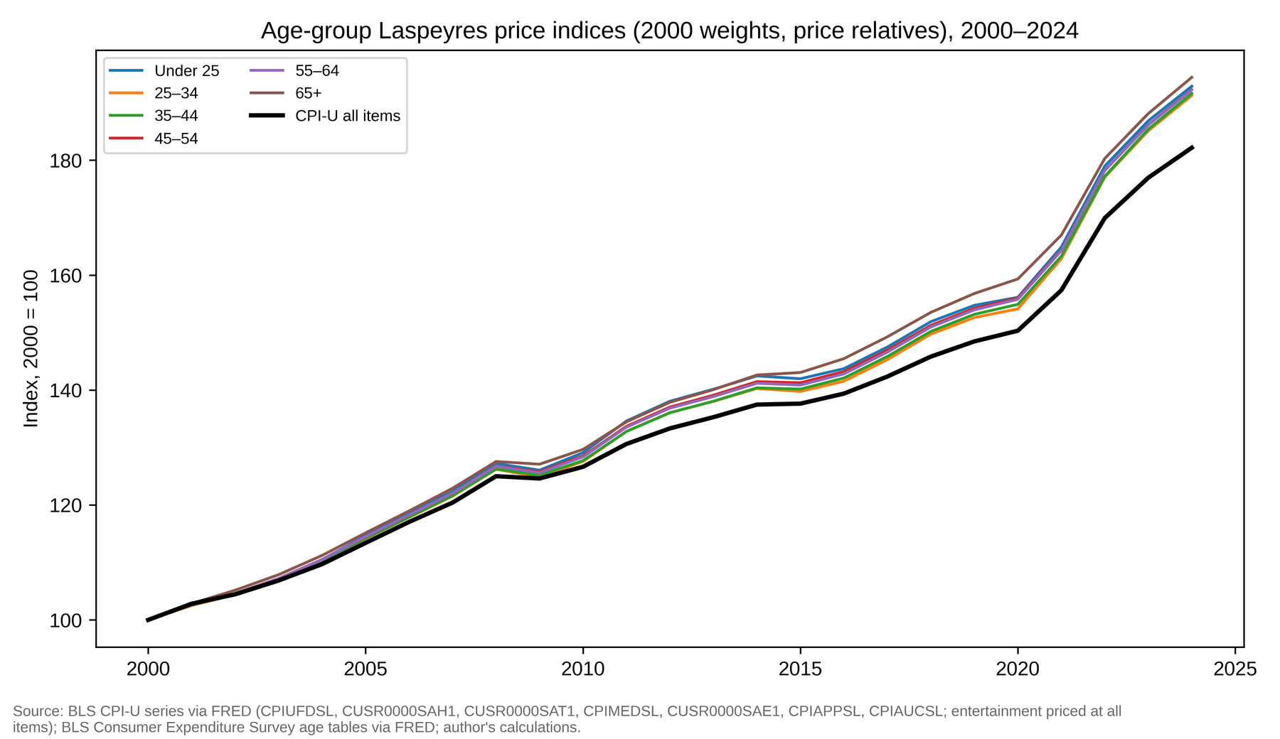
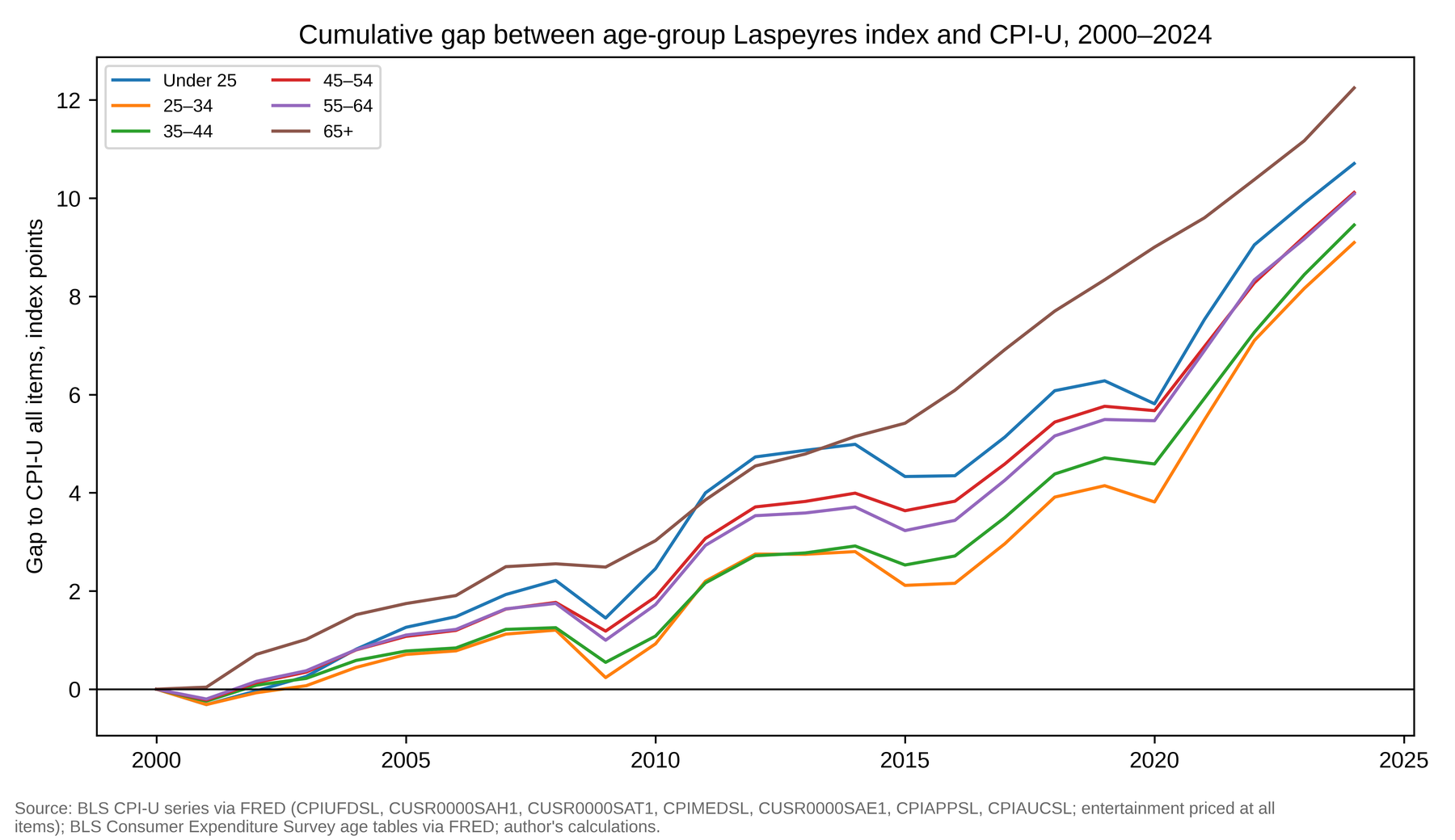
Figure 1 plots the six headline indices against the all-items CPI-U and Figure 2 the gaps. In 2024 the indices ranged from 191.28 (25–34) to 194.43 (65 and over) against 182.18 for the aggregate (Table 1). The gaps are small in the 2000s (in 2001 all six were within ±0.3 point of zero, five of them negative), grow after 2010, dip in 2009 and 2020 when transportation prices fell, and widen in 2021–2024.
| Age group | Laspeyres | Paasche | Chained L | Chained P | Gap Gᴸ | Gap, chained L |
|---|---|---|---|---|---|---|
| Under 25 | 192.88 | 192.84 | 194.43 | 192.14 | 10.71 | 12.25 |
| 25–34 | 191.28 | 191.55 | 191.76 | 190.45 | 9.10 | 9.58 |
| 35–44 | 191.63 | 191.53 | 191.78 | 190.88 | 9.45 | 9.60 |
| 45–54 | 192.30 | 192.59 | 192.65 | 191.18 | 10.12 | 10.47 |
| 55–64 | 192.27 | 192.69 | 192.44 | 190.99 | 10.09 | 10.26 |
| 65 and over | 194.43 | 194.36 | 194.23 | 193.02 | 12.25 | 12.05 |
All-items CPI-U index 182.18 (annual average 313.70, 1982–84 = 100).
5.2 The age profile of the gap
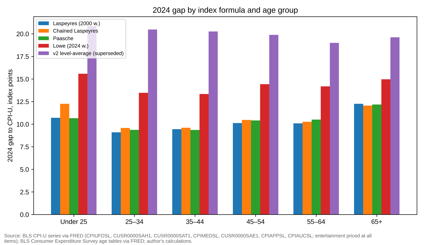
Table S1 in the Online Appendix reports the headline gap in every year and Table 2 the 2024 gap under every formula. Three findings. First, the 65-and-over group has the largest headline gap in every year from 2001 and the largest period mean (4.91 points against 2.58–3.97 for the others), so Hypothesis H1 is supported. Second, the 2024 profile is U-shaped under the headline index (10.71, 9.10, 9.45, 10.12, 10.09, 12.25), under Paasche (10.66, 9.37, 9.36, 10.41, 10.51, 12.18), under chained Laspeyres (12.25, 9.58, 9.60, 10.47, 10.26, 12.05, with the under-25 group at the top), under chained Paasche and under both Lowe baskets. The earlier draft reported that the young end of the U “does not survive fixed-base weighting”; that conclusion was an artefact of the level-average construct and of the pension-inclusive denominator, and is withdrawn. Hypothesis H2 is supported. Third, the between-group spread is modest: 3.15 points in 2024 (headline), 2.67 (chained L), 3.53 (Paasche), against a common excess of 9–12 points that reflects the mapping. Medical services versus commodities. The oldest group’s position depends on which medical prices it faces. Priced at medical-care services (relative 2.302) its gap rises to 14.02 and the spread to 4.43; priced at medical commodities (1.734, the slowest-rising component other than apparel) its gap falls to 6.81, the lowest of the six, and the U inverts at the old end. CE aggregate tables do not split medical spending by age into services and drugs, so the headline uses the aggregate index; the composition of older households’ medical spending is therefore the main unresolved input.
| Age group | Laspeyres | Paasche | Chained L | Chained P | Lowe 2024 | Lowe mean | Med. services | Med. commod. |
|---|---|---|---|---|---|---|---|---|
| Under 25 | 10.71 | 10.66 | 12.25 | 9.96 | 15.58 | 14.56 | 11.04 | 9.69 |
| 25–34 | 9.10 | 9.37 | 9.58 | 8.27 | 13.47 | 11.77 | 9.59 | 7.57 |
| 35–44 | 9.45 | 9.36 | 9.60 | 8.70 | 13.34 | 11.91 | 10.06 | 7.58 |
| 45–54 | 10.12 | 10.41 | 10.47 | 9.00 | 14.43 | 13.25 | 10.86 | 7.84 |
| 55–64 | 10.09 | 10.51 | 10.26 | 8.81 | 14.18 | 12.86 | 11.08 | 7.06 |
| 65 and over | 12.25 | 12.18 | 12.05 | 10.84 | 14.97 | 13.94 | 14.02 | 6.81 |
| Spread | 3.15 | 3.53 | 2.67 | 2.57 | 2.24 | 2.79 | 4.43 | 2.88 |
Med. services / commod.: headline Laspeyres with the aggregate medical relative replaced by CUUR0000SAM2 or CUUR0000SAM1. With shares over total expenditure (the earlier draft’s denominator) the Laspeyres gaps are 10.13, 8.25, 8.50, 9.07, 9.10, 11.81. Figure 3 plots the columns.
5.3 Sampling error of the indices
Table S5 in the Online Appendix reports the share-error bootstrap. Sampling error in the CE means is not negligible for the under-25 group, whose 2024 headline gap has a 95 per cent interval of 8.7 to 12.8 points (standard deviation 1.03) against 0.3–0.5 for the other groups; the 65-and-over gap lies between 11.4 and 13.2. The ordinal findings survive: the 65-and-over group has the largest headline gap in 91 per cent of replications (96 per cent with correlated errors), the profile is U-shaped, with both ends above their neighbours, in 87 per cent (95 per cent), and under the chained Laspeyres the two ends are the two highest groups in 95 per cent (99 per cent). The cohort differential is estimated far more precisely than its size might suggest: its 95 per cent intervals, 0.17–0.21 points a year for the least-affected cohort and 0.23–0.28 for the cohort that started under 25, exclude zero by more than twenty standard deviations, because share error perturbs a weighted average of relatives whose spread is fixed. The one statistic that is imprecise is the between-group spread, 2.3–4.4 points (headline) and 2.1–4.9 (chained), most of it from the under-25 group.
5.4 Finer category resolution
Table 3 recomputes the 2024 gaps with twenty-four categories. The common excess over the CPI-U falls, as expected once the seven-category compromises (housing at shelter, medical care at the aggregate, entertainment and the residual at all items) are replaced by item indices: the headline gaps fall by 2.1–3.8 points and the chained gaps by 5.2–6.9 points. What does not change is the shape. Under the fixed-base index the 65-and-over group remains highest (9.72) and the under-25 group second (8.21); under the chained index the under-25 group is highest (7.01) and the 65-and-over group second (6.55); the two ends of the age distribution are the two highest groups under both formulas, the Spearman rank correlations with the seven-category gaps are 0.83 (fixed-base) and 0.94 (chained), and the between-group spread is if anything wider, 3.46 and 4.06 points against 3.15 and 2.67. The seven-category mapping therefore overstates the level of every group’s excess inflation but not the ordering that the paper’s conclusions rest on.
| Age group | Headline (fixed-2000 L), 7 categories | Headline (fixed-2000 L), 24 categories | Chained Laspeyres, 7 categories | Chained Laspeyres, 24 categories |
|---|---|---|---|---|
| Under 25 | 10.71 | 8.21 | 12.25 | 7.01 |
| 25–34 | 9.10 | 6.52 | 9.58 | 3.02 |
| 35–44 | 9.45 | 6.93 | 9.60 | 2.95 |
| 45–54 | 10.12 | 8.02 | 10.47 | 4.82 |
| 55–64 | 10.09 | 6.26 | 10.26 | 3.38 |
| 65 and over | 12.25 | 9.72 | 12.05 | 6.55 |
| Spread | 3.15 | 3.46 | 2.67 | 4.06 |
Notes: CE detailed means from the standard-error tables (U.S. Bureau of Labor Statistics, 2013, 2025); shares over outlays excluding pensions. CPI-U series (NSA, U.S. city average, annual averages): food at home SAF11, food away SEFV, alcohol SAF116, shelter SAH1, utilities SAH2, household operations SEHP, housekeeping supplies SAH31 (from 2009, back-cast with SAH3), furnishings SAH3, apparel SAA, vehicle purchases SETA, gasoline SETB, other vehicle expenses geometric mean of maintenance SETD and insurance SETE, public transportation SETG, health insurance and medical services SAM2 (the CPI health-insurance index measures insurers’ retained earnings and starts in 2005), prescription drugs SEMF and medical supplies SEMG (from 2009, back-cast with medical commodities SAM1), entertainment SAR, education SAE1, personal care SAG1, reading SERG, tobacco SEGA, miscellaneous SAG, cash contributions at all items. Eight suppressed detailed cells (all in 2022–2023, six of them under 25) receive zero weight, so their outlay is priced at the all-items index. The 2024 household-operations value is the average of the six published bimonthly values.
5.5 Konüs bounds and substitution
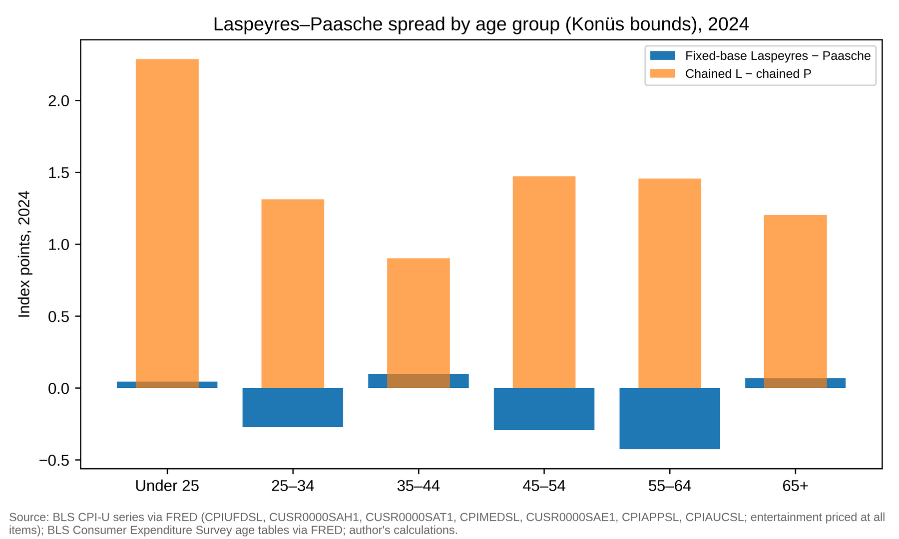
Table 1 gives the Laspeyres–Paasche spread in 2024. With fixed 2000 and 2024 baskets it is between −0.43 and +0.10 index points for every group, and negative for three, so at seven-category resolution there is no detectable substitution away from faster-rising categories for any age group over 24 years: the shares moved, but not systematically towards the cheaper categories. The chained spread (chained L minus chained P) is positive for all groups, 2.29 (under 25), 1.31, 0.90, 1.47, 1.46 and 1.20 (65 and over); it is largest for the youngest group and smallest for the 35–44 group, not for the oldest. Hypothesis H4, which predicted the smallest spread for the 65-and-over group on low-substitutability grounds, is not supported (Figure 4). The synthetic-cohort indices of Section 5.7 are chained Laspeyres only, so for them no Paasche counterpart and no bound is available. The chained spread, moreover, mixes substitution with chain drift, and the excess of the chained over the fixed-base Laspeyres for the under-25 group (12.25 against 10.71) is consistent with chain drift in the group whose shares are the noisiest.
5.6 Expenditure-share decomposition
Because the headline gap is linear in the base shares, it decomposes exactly: Gᴸₐ,2024 = 100 ∑ᵢ wₐ,ᵢ,2000 (Rᵢ,2024 − Rᴬ2024), with the residual contributing zero. Table 4 reports the result.
| Age group | Food | Housing | Transport. | Health care | Education | Apparel | Total |
|---|---|---|---|---|---|---|---|
| Under 25 | 2.20 | 8.33 | −0.22 | 0.80 | 4.96 | −5.37 | 10.71 |
| 25–34 | 2.18 | 9.23 | −0.22 | 1.21 | 1.39 | −4.70 | 9.10 |
| 35–44 | 2.20 | 9.31 | −0.20 | 1.49 | 1.28 | −4.62 | 9.45 |
| 45–54 | 2.23 | 8.57 | −0.20 | 1.81 | 2.33 | −4.63 | 10.12 |
| 55–64 | 2.13 | 8.71 | −0.20 | 2.41 | 0.90 | −3.85 | 10.09 |
| 65 and over | 2.09 | 8.56 | −0.16 | 4.32 | 0.36 | −2.92 | 12.25 |
Component relatives 2024 (2000 = 1): food 1.968, housing (shelter) 2.072, transportation 1.813, health 2.162, education 2.663, apparel 1.015, all items 1.822. Base (2000) shares in the Online Appendix, Table S2.
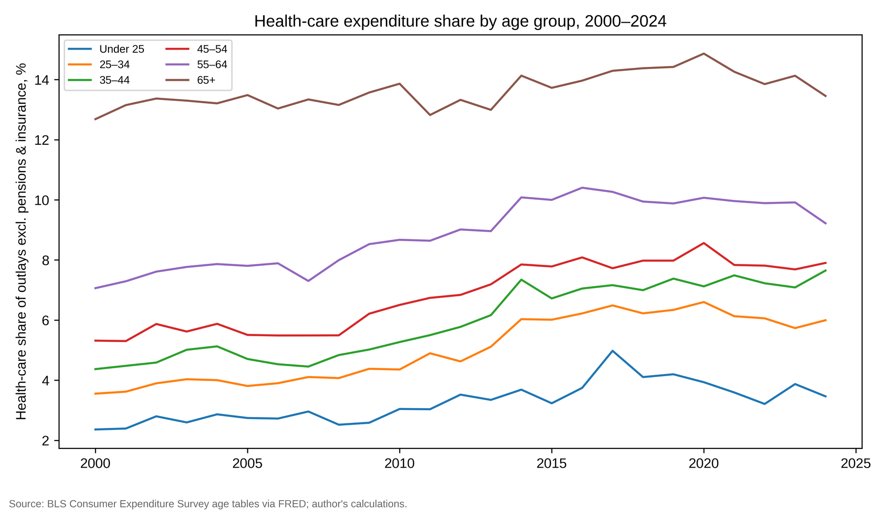
Housing contributes 8.3–9.3 points to every group and is the reason all six gaps are positive; it is largest for the 25–44 groups, whose housing shares (36.9–37.2 per cent excluding pensions) are the highest. Different expenditure categories account for the two ends of the U. The under-25 group’s education share (5.9 per cent in 2000) contributes 4.96 points, more than its offset from a large apparel share (−5.37, apparel having barely risen). The 65-and-over group’s health-care share (12.7 per cent) contributes 4.32 points, against 0.80–2.41 for the others, and its low apparel share means the smallest apparel offset. The middle groups have the smallest combined education and health contributions, which produces the trough. Figure 5 shows the health share over time; it rises with age in every year and rose within every group, most for 35–54.
5.7 Synthetic birth cohorts
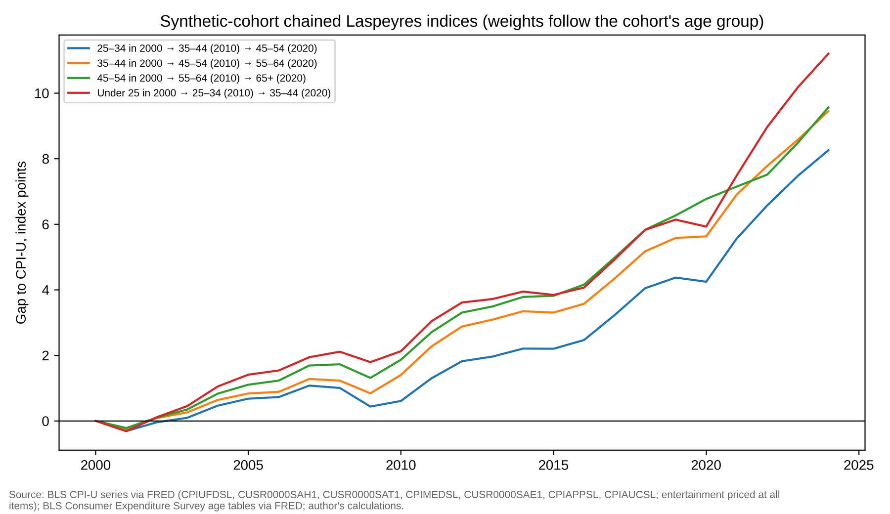
To move from age groups towards cohorts, four synthetic cohorts were chained through the age groups: a cohort aged 25–34 in 2000 takes that group’s weights for 2000–2009, the 35–44 weights for 2010–2019 and the 45–54 weights for 2020–2024, and so on (Table 5, Figure 6). Each cohort’s 2024 index lies within 0.3–1.3 points of the stayer index of its starting group, and every cohort experienced annualised inflation of 2.72–2.79 per cent against 2.53 per cent for the all-items index. The cohort that started under 25 fared worst (193.38, gap 11.20), because it carried the education exposure of youth and then the housing exposure of the 25–44 years. The paths do not separate age, period and cohort effects (Bell & Jones, 2014; Ryder, 1965); they show that the age-group results are not overturned when weights follow a cohort rather than a stage.
| Cohort (age in 2000 → 2010 → 2020) | 2024 index | Gap | Stayer gap | Annualised (%) |
|---|---|---|---|---|
| Under 25 → 25–34 → 35–44 | 193.38 | 11.20 | 12.25 | 2.786 |
| 25–34 → 35–44 → 45–54 | 190.43 | 8.25 | 9.58 | 2.720 |
| 35–44 → 45–54 → 55–64 | 191.63 | 9.45 | 9.60 | 2.747 |
| 45–54 → 55–64 → 65+ | 191.74 | 9.56 | 10.47 | 2.749 |
| All-items CPI-U | 182.18 | 2.531 |
Stayer gap: chained Laspeyres gap of the cohort’s starting age group in 2024.
5.8 Homeownership regressions
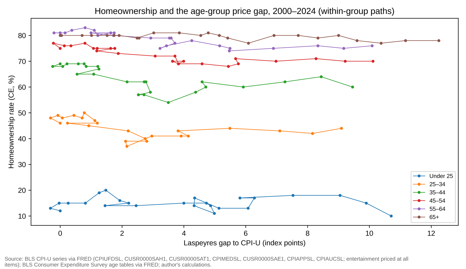
Table 6 reports the estimates. With age fixed effects alone the slope is −0.51 (p < 0.001), replicating the earlier draft’s negative finding. Adding year fixed effects reverses the sign: +2.03, HC1 s.e. 0.34, cluster-by-age s.e. 0.60 (p = 0.001 asymptotic; wild-cluster bootstrap p = 0.016 with enumerated Rademacher weights and 0.027 with Webb weights), R² = 0.994, DW 1.73. The same reversal holds with the chained gap (+2.65) and with total-expenditure shares (+1.99). The within-group models tell the same story: bivariate slopes are negative and nominally significant for the 25–64 groups, but with DW of 0.28–0.73; adding the all-items index or a linear trend turns the slopes positive for the 25–54 groups (significantly so at 25–44), and in first differences no slope differs from zero at the 10 per cent level. The negative age-FE coefficient therefore reflects the common downward path of homeownership after 2006 coinciding with the common upward path of the gap, rather than a within-group relationship. Hypothesis H3 is not supported, as no negative within-group association is detectable once common time effects are removed and the point estimates with time controls are positive. A positive two-way coefficient has an interpretation the paper does not press: groups whose homeownership held up best (55 and over) are also those whose health-care exposure rose fastest, and homeownership itself lowers a group’s measured shelter share, so the sign may be partly compositional. The health-share models for the 55–64 group show a negative association (−2.76 points of homeownership per percentage point of health share, DW 0.97) that weakens to −1.85 with the all-items index; for the 65-and-over group there is none. These are two trending series in 25 observations and are reported for completeness.
| Model | Coef. on gap | HC1 SE | p | R² | N | DW |
|---|---|---|---|---|---|---|
| Pooled OLS | −0.1654 | 0.643 | 0.797 | 0.0005 | 150 | 1.667 |
| Age fixed effects | −0.5052 | 0.065 | <0.001 | 0.987 | 150 | 1.011 |
| Two-way fixed effects (age + year) | +2.0313 | 0.342 | <0.001 | 0.994 | 150 | 1.726 |
| cluster-by-age SE | 0.600 | 0.001 | ||||
| wild-cluster bootstrap p (Rademacher, 64 / Webb, 9,999) | 0.016 / 0.027 | |||||
| Two-way FE, chained-L gap | +2.6497 | 0.399 | <0.001 | 0.995 | 150 | 1.753 |
| cluster SE / wild-bootstrap p (Webb) | 0.521 | 0.038 | ||||
| Two-way FE, total-expenditure shares | +1.9931 | 0.325 | <0.001 | 0.994 | 150 | 1.740 |
| cluster SE / wild-bootstrap p (Webb) | 0.611 | 0.028 | ||||
| Within group: bivariate / + all-items index / + linear trend / first differences (coefficient, p) | ||||||
| Under 25 | −0.048 (0.81) / −0.895 (0.32) / −0.734 (0.23) / −0.646 (0.28) | |||||
| 25–34 | −0.659 (0.006) / +2.167 (0.028) / +1.223 (0.003) / −0.222 (0.60) | |||||
| 35–44 | −0.959 (0.001) / +2.775 (0.013) / +1.846 (0.001) / +0.258 (0.76) | |||||
| 45–54 | −0.771 (<0.001) / +0.052 (0.94) / +0.783 (0.010) / −0.362 (0.46) | |||||
| 55–64 | −0.785 (<0.001) / +0.206 (0.78) / +0.343 (0.24) / +0.595 (0.14) | |||||
| 65 and over | −0.176 (<0.001) / +0.029 (0.92) / −0.434 (0.13) / +0.209 (0.74) | |||||
| Health-care share models (homeownership on health share in percentage points) | ||||||
| 55–64, bivariate | −2.764 | 0.307 | <0.001 | 0.793 | 25 | 0.974 |
| 55–64, + all-items index | −1.848 | 0.367 | <0.001 | 0.851 | 25 | 1.176 |
| 65 and over, bivariate | −0.716 | 0.444 | 0.107 | 0.092 | 25 | 1.241 |
| 65 and over, + all-items index | +0.038 | 0.556 | 0.945 | 0.343 | 25 | 1.479 |
Within-group bivariate DW: 0.985, 0.278, 0.296, 0.404, 0.726, 1.484; first-difference DW 1.69–2.50. Cluster-robust inference with six clusters is indicative only. Figure 7 shows the scatter.
5.9 Summary of hypothesis tests
H1 (oldest group largest gap): supported under the headline, Paasche, both Lowe and the medical-services variants; under chained Laspeyres the under-25 group is 0.2 point higher; reversed under the medical-commodities variant; holds in 91–96 per cent of share-error bootstrap replications, and under the twenty-four-category mapping for the fixed-base index (under the chained index the under-25 group is highest). H2 (U-shape): supported under every formula, under the twenty-four-category mapping, and in 87–100 per cent of share-error bootstrap replications. H3 (negative within-group association with homeownership): not supported once year effects are included. H4 (smallest substitution bound for the oldest): not supported.
6 Discussion
6.1 The U-shape and what drives it
The exposure of American households to component price growth since 2000 has been greatest at the two ends of the age distribution, for different reasons: the old through medical care, the young through education and a housing share that is high at every age under 45. The middle-aged groups have the lowest exposure because they combine a moderate housing share with small education and health shares. The result is robust to formula, which the earlier draft’s level-average construct had obscured. The between-group differences are nonetheless second-order beside the common excess of 9–12 points, which is largely the shelter mapping, and beside the within-group dispersion that microdata reveal (Kaplan & Schulhofer-Wohl, 2017).
6.2 Substitution and capability
The capability argument of Section 2 predicted that older households, whose baskets are dominated by low-substitutability goods, would show the smallest Laspeyres–Paasche spread. They do not; at seven-category resolution no group shows a fixed-base spread distinguishable from zero, and the chained spread is largest for the young. Either substitution across major categories is negligible at every age, so the capability argument is about within-category substitution the data cannot see, or the CE aggregate shares are too coarse and too noisy to reveal it. The paper cannot tell which, and records the null.
6.3 Homeownership: a withdrawn result
The earlier draft reported that within age groups, years of higher excess inflation were years of lower homeownership for ages 25–64. Section 5.8 shows this to be a period effect: once year fixed effects absorb the housing bust and the credit cycle, the coefficient is positive. The life-course mechanism, by which price disadvantage in the household-formation years compounds through delayed entry, is not refuted by this, since the test has neither age-specific income and credit controls nor a cohort design, but the paper no longer claims empirical support for it. The synthetic-cohort paths, which show cohorts entering adulthood after 2000 facing 0.2–0.25 percentage points a year more inflation than the aggregate, are the closest the data come to the compounding claim.
6.4 External benchmark: the BLS R-CPI-E
The natural check on the 65-and-over result is the BLS R-CPI-E (n.d.-k), which applies the same reweighting logic to roughly 200 item strata for consumer units whose reference person or spouse is 62 or older. The monthly series (December 1982 = 100) was downloaded from the BLS research-series page on 24 September 2026, averaged to annual frequency and rebased to 2000 = 100. Over 2000–2024 the R-CPI-E rose 86.7 per cent against 82.2 per cent for the CPI-U, an annualised 2.63 against 2.53 per cent, a cumulative excess of 4.5 index points and a mean annual excess of 0.10 percentage points. This is about half the 0.2 points a year that the BLS reported for 1982–2007 (Amble & Stewart, 1994; Stewart, 2008).
The raw 65-and-over gap in Table 1 (12.25 points) is not the comparable quantity, because, as Section 4 explains, most of every group’s gap to the CPI-U is a mapping effect shared by all groups (housing priced at shelter, apparel at goods only). The comparable quantity is the 65-and-over index relative to the other groups under the same method. Table 7 sets the two side by side. The 65-and-over excess over the mean of the 25–64 groups was 2.6 points in 2024 and peaked at 4.1 points in 2020; the R-CPI-E excess over the CPI-U was 4.5 and 3.7 points in the same years. The year-on-year excesses have the same sign in 19 of 24 years (correlation 0.73). The seven-category method therefore reproduces the sign, timing and order of magnitude of the official research index, although it understates its size by about a third to a half in recent years. This is the expected direction, because within-category composition that the coarse mapping cannot see (owners’ equivalent rent within shelter, the medical care mix, the 62-and-over versus 65-and-over population) works in the same direction as the between-category weights.
| 2005 | 2010 | 2015 | 2020 | 2022 | 2024 | |
|---|---|---|---|---|---|---|
| R-CPI-E − CPI-U (BLS) | 1.27 | 1.43 | 2.28 | 3.65 | 2.84 | 4.47 |
| 65+ − CPI-U (this paper, Laspeyres) | 1.74 | 3.03 | 5.42 | 9.00 | 10.38 | 12.25 |
| 65+ − mean of 25–64 groups | 0.83 | 1.62 | 2.54 | 4.12 | 2.63 | 2.56 |
| 65+ − 25–34 | 1.04 | 2.10 | 3.30 | 5.19 | 3.28 | 3.15 |
Sources: BLS R-CPI-E data file (r-cpi-e-data.xlsx, accessed 24 September 2026) (U.S. Bureau of Labor Statistics, n.d.-k); CPI-U all items (CPIAUCSL) (U.S. Bureau of Labor Statistics, n.d.-b); author’s calculations. The R-CPI-E population is 62 and over; the paper’s is 65 and over. The second row is not comparable with the first because the mapping effect described in Section 4 is common to all age groups.
The UK Household Costs Indices (2026) show retired-versus-non-retired differences of 0.1 point in early 2026, which illustrates that group differences in inflation are typically small in any one year and matter through accumulation.
6.5 Limitations
1. Aggregate rather than micro data. Published CE means by age group, not PUMD; within-group heterogeneity is invisible. Sampling error in the published means is, however, quantified: the share-error bootstrap of Section 5.3, built on the BLS standard-error tables for 2000–2024 (U.S. Bureau of Labor Statistics, 2013, 2025), gives the 65-and-over gap a 95 per cent interval of 11.4–13.2 points and the under-25 gap 8.7–12.8, and reproduces the U-shape in 87–100 per cent of replications. What it cannot capture is heterogeneity within an age group, or the non-sampling error discussed in item 5.
2. Category granularity and mapping. Seven categories; CE housing priced at CPI shelter, CE apparel and services at CPI apparel (goods only), medical care at the aggregate index. These bias the level of all gaps and, as the medical variant shows, can bias differences. Section 5.4 recomputes the gaps with twenty-four categories: the level of every gap falls by 2–7 points, the ordering does not change. The finer mapping has compromises of its own (other vehicle expenses, health insurance, cash contributions), so it is reported as a robustness check rather than adopted as the headline.
3. Entertainment and residual priced at the all-items index; residual shares (excluding pensions) range from 7.2 to 13.4 per cent in 2000.
4. Chained indices fail time reversal and drift; the under-25 chained series is the most affected.
5. CE measurement error varies by category and has grown over time (Bee et al., 2015; Passero et al., 2015); the under-25 group is the smallest sample and its shares the noisiest. The cohort differential of 0.19–0.26 percentage points a year is small, but it is robust to share error of plausible size: with medical care growing 0.74 points a year faster than the all-items index, shelter 0.55 and education 1.64 (2000–2024, Table S4 in the Online Appendix), a one-point error in a base-period share moves the annualised index by at most 0.016 points, and erasing the smallest cohort differential would require a share error of about 25 points in medical care or 12 points in education, an order of magnitude beyond the between-group share differences themselves. This bound treats one share at a time; correlated errors across several shares in the same direction would tighten it, which is why the bootstrap of Section 5.3 includes a correlated-error variant, under which the cohort-differential intervals (0.18–0.20 and 0.23–0.27) are, if anything, narrower. The bound and the bootstrap address sampling error; systematic under-reporting of particular categories (Bee et al., 2015; Passero et al., 2015) is not captured by either.
6. Consumer units, not individuals; age of reference person.
7. Age groups, not cohorts; the synthetic cohorts are a construction, not observed households (Bell & Jones, 2014).
8. External benchmark. The R-CPI-E confirms the sign and order of magnitude of the 65-and-over excess, but the between-group excess measured here is about a third to a half smaller than the R-CPI-E excess in recent years; the difference is a measure of what the seven-category mapping misses.
9. Regressions. Twenty-five annual observations per group, trending series, six clusters (the wild-cluster bootstrap moves the two-way p-value from 0.001 to 0.02–0.03 depending on the weight distribution, Table 6), no age-specific income or credit controls; nothing is causal.
10. Integer homeownership rates from a survey sample.
11. No cross-national comparison beyond the qualitative ONS reference. The euro-area household-group inflation work of the European Central Bank, which prices HICP components against income-group expenditure shares (Charalampakis et al., 2022), uses the same shares-times-relatives construction and is the natural comparator for a European age-group extension.
7 Policy Implications
An official set of age-specific indices. The BLS already produces the R-CPI-E for households aged 62 and over (Stewart, 2008; U.S. Bureau of Labor Statistics, n.d.-k). A full set of age-specific indices from the CE and CPI components would be cheap to produce, and the youngest group, whose gap is as large as the oldest group’s under every formula, merits a dedicated series. Publication should be in fixed-base and chained forms, with the medical services/commodities split by age, since that split decides the oldest group’s ranking.
Indexation. Social Security benefits are indexed to the CPI-W, whose weights are those of urban wage-earner and clerical-worker households (U.S. Bureau of Labor Statistics, n.d.-j). The 65-and-over group has the largest headline gap here, but the difference from the aggregate is about 0.3 points a year and whether a CPI-E should replace the CPI-W is a question of fiscal cost, of the medical composition just noted, and of the balance-sheet channel (Auclert, 2019; Doepke & Schneider, 2006) as much as of measurement.
Housing. Housing is the largest contributor to every group’s gap and the largest for ages 25–44. Policies that lower the entry cost of homeownership address the component that drives the common excess.
Statistical infrastructure. Publishing CE age tables with consumer-unit counts, standard errors and a medical services/commodities split, and adding the R-CPI-E to the public API (it is currently released only as a spreadsheet), would remove several of the limitations listed above.
8 Conclusions
This paper constructed age-group-specific Laspeyres price indices for the United States over 2000–2024 from public data, bounded them with Paasche and chained variants, decomposed the 2024 gaps exactly by category, followed four synthetic cohorts, and related the gaps to homeownership. The findings that hold under every formula are the U-shaped age profile of excess inflation, driven by education and housing for the young and by medical care for the old, and the position of the 65-and-over and under-25 groups at the top. Three earlier conclusions are withdrawn: that the young end of the U was a weighting artefact (it is not); that within-group inflation gaps were negatively associated with homeownership (they are not, once year effects are removed); and the headline construct itself, which failed commensurability. The between-group differences within the CPI’s own basket are modest, and they are only one part of what a statistical system would need in order to describe the material conditions of different generations.
Statements and Declarations
Data availability. All data are publicly available from FRED (Consumer Expenditure Surveys release 479; CPI-U series CPIUFDSL, CUSR0000SAH1, CUSR0000SAT1, CPIMEDSL, CUSR0000SAE1, CPIAPPSL, CPIAUCSL, CUUR0000SAM1, CUUR0000SAM2), from the BLS research-series page (R-CPI-E), from the BLS Consumer Expenditure Survey standard-error tables by age of reference person for 2000–2011 and 2012–2024 (U.S. Bureau of Labor Statistics, 2013, 2025), and, for the twenty-four-category mapping, from the CPI-U item series listed in the note to Table 3 (retrieved through the FRED and BLS public APIs). The constructed panel, the R-CPI-E comparison, index series under every formula, decomposition, synthetic-cohort paths, regression output, the parsed standard-error tables, the bootstrap draws and the replication scripts will be deposited in a public repository; until then they are available from the author on request.
Competing interests. The author has no relevant financial or non-financial interests to disclose.
Funding. No funding was received for conducting this study.
Ethics approval. Only published aggregate statistics were used; the study involved no human participants and no individual-level data, and ethics approval was not required.
Use of large language models. A large language model (Claude, Anthropic, accessed through the Abacus.AI platform) was used to interpret statistical output and to verify data accuracy. All underlying data were supplied directly to the model to avoid hallucinated numbers. The model is not an author.
Data appendix
The Online Appendix (pages 26 to 28 of the PDF) accompanies the manuscript and contains the full annual gap series, the base-period expenditure shares, and the superseded index construction referred to in the main text. Table S1, the headline cohort CPI gap by age group in every year (index points), is reproduced here.
| Year | Under 25 | 25–34 | 35–44 | 45–54 | 55–64 | 65+ | All-items index |
|---|---|---|---|---|---|---|---|
| 2000 | 0.00 | 0.00 | 0.00 | 0.00 | 0.00 | 0.00 | 100.00 |
| 2001 | −0.31 | −0.31 | −0.24 | −0.22 | −0.20 | 0.04 | 102.82 |
| 2002 | −0.03 | −0.07 | 0.08 | 0.14 | 0.16 | 0.71 | 104.46 |
| 2003 | 0.26 | 0.07 | 0.22 | 0.35 | 0.38 | 1.02 | 106.86 |
| 2004 | 0.81 | 0.44 | 0.59 | 0.80 | 0.81 | 1.52 | 109.71 |
| 2005 | 1.26 | 0.71 | 0.78 | 1.08 | 1.10 | 1.74 | 113.40 |
| 2006 | 1.48 | 0.78 | 0.84 | 1.20 | 1.22 | 1.91 | 117.05 |
| 2007 | 1.93 | 1.12 | 1.22 | 1.63 | 1.64 | 2.50 | 120.41 |
| 2008 | 2.22 | 1.20 | 1.25 | 1.77 | 1.75 | 2.55 | 125.01 |
| 2009 | 1.45 | 0.24 | 0.55 | 1.18 | 1.00 | 2.49 | 124.61 |
| 2010 | 2.45 | 0.92 | 1.08 | 1.88 | 1.72 | 3.03 | 126.65 |
| 2011 | 4.00 | 2.20 | 2.17 | 3.07 | 2.93 | 3.86 | 130.62 |
| 2012 | 4.73 | 2.75 | 2.72 | 3.71 | 3.53 | 4.55 | 133.33 |
| 2013 | 4.87 | 2.75 | 2.78 | 3.82 | 3.59 | 4.79 | 135.29 |
| 2014 | 4.99 | 2.80 | 2.92 | 3.99 | 3.71 | 5.15 | 137.47 |
| 2015 | 4.33 | 2.11 | 2.53 | 3.63 | 3.23 | 5.42 | 137.64 |
| 2016 | 4.35 | 2.16 | 2.71 | 3.83 | 3.44 | 6.09 | 139.38 |
| 2017 | 5.13 | 2.96 | 3.50 | 4.59 | 4.25 | 6.92 | 142.35 |
| 2018 | 6.08 | 3.91 | 4.38 | 5.44 | 5.16 | 7.70 | 145.83 |
| 2019 | 6.28 | 4.14 | 4.71 | 5.76 | 5.49 | 8.34 | 148.47 |
| 2020 | 5.81 | 3.81 | 4.59 | 5.67 | 5.47 | 9.00 | 150.33 |
| 2021 | 7.53 | 5.49 | 5.92 | 6.98 | 6.90 | 9.60 | 157.37 |
| 2022 | 9.05 | 7.10 | 7.27 | 8.28 | 8.34 | 10.38 | 169.94 |
| 2023 | 9.90 | 8.16 | 8.44 | 9.22 | 9.17 | 11.17 | 176.96 |
| 2024 | 10.70 | 9.10 | 9.45 | 10.12 | 10.09 | 12.25 | 182.18 |
The remaining supplementary tables are in the PDF: Table S2 (base-period 2000 shares of outlays excluding personal insurance and pensions, and pension shares of total expenditure), Table S3 (summary statistics by age group, 2000–2024), Table S4 (CPI-U component growth, 2000–2024 annual averages) and Table S5 (share-error bootstrap, 2,000 replications of the CE means from their published standard errors), together with Section S2 on the superseded construction used in the earlier draft.
References
- [1]Amble, N., & Stewart, K. (1994). Experimental price index for elderly consumers. Monthly Labor Review, 117(5), 11–16.
- [2]Argente, D., & Lee, M. (2021). Cost of living inequality during the Great Recession. Journal of the European Economic Association, 19(2), 913–952. https://doi.org/10.1093/jeea/jvaa018
- [3]Auclert, A. (2019). Monetary policy and the redistribution channel. American Economic Review, 109(6), 2333–2367. https://doi.org/10.1257/aer.20160137
- [4]Auerbach, A. J., Gokhale, J., & Kotlikoff, L. J. (1991). Generational accounts: A meaningful alternative to deficit accounting. Tax Policy and the Economy, 5, 55–110. https://doi.org/10.1086/tpe.5.20061801
- [5]Bee, A., Meyer, B. D., & Sullivan, J. X. (2015). The validity of consumption data: Are the CE and PSID consumption data informative about consumption trends? In C. D. Carroll, T. F. Crossley, & J. Sabelhaus (Eds.), Improving the measurement of consumer expenditures. University of Chicago Press.
- [6]Bell, A., & Jones, K. (2014). Another ‘futile quest’? A simulation study of Yang and Land’s hierarchical age-period-cohort model. Demographic Research, 30, 333–360. https://doi.org/10.4054/demres.2014.30.11
- [7]Boskin, M. J., Dulberger, E. R., Gordon, R. J., Griliches, Z., & Jorgenson, D. W. (1996). Toward a more accurate measure of the cost of living: Final report to the Senate Finance Committee (tech. rep.). Advisory Commission to Study the Consumer Price Index. Washington, DC.
- [8]Boskin, M. J., Dulberger, E. R., Gordon, R. J., Griliches, Z., & Jorgenson, D. W. (1998). Consumer prices, the consumer price index, and the cost of living. Journal of Economic Perspectives, 12(1), 3–26. https://doi.org/10.1257/jep.12.1.3
- [9]Cameron, A. C., Gelbach, J. B., & Miller, D. L. (2008). Bootstrap-based improvements for inference with clustered errors. Review of Economics and Statistics, 90(3), 414–427. https://doi.org/10.1162/rest.90.3.414
- [10]Charalampakis, E., Fagandini, B., Henkel, L., & Osbat, C. (2022). The impact of the recent rise in inflation on low-income households. ECB Economic Bulletin, 7/2022. Retrieved September 24, 2026, from https://www.ecb.europa.eu/press/economic-bulletin/focus/2022/html/ecb.ebbox202207_04~a89ec1a6fe.en.html
- [11]Chetty, R., Grusky, D., Hell, M., Hendren, N., Manduca, R., & Narang, J. (2017). The fading American dream: Trends in absolute income mobility since 1940. Science, 356(6336), 398–406. https://doi.org/10.1126/science.aal4617
- [12]Cravino, J., Lan, T., & Levchenko, A. A. (2020). Price stickiness along the income distribution and the effects of monetary policy. Journal of Monetary Economics, 110, 19–32. https://doi.org/10.1016/j.jmoneco.2018.12.001
- [13]Crawford, I., & Oldfield, Z. (2002). Distributional aspects of inflation (IFS Commentary No. 90). Institute for Fiscal Studies. London.
- [14]Dannefer, D. (2003). Cumulative advantage/disadvantage and the life course: Cross-fertilizing age and social science theory. The Journals of Gerontology Series B: Psychological Sciences and Social Sciences, 58(6), S327–S337. https://doi.org/10.1093/geronb/58.6.s327
- [15]Diewert, W. E. (1976). Exact and superlative index numbers. Journal of Econometrics, 4(2), 115–145. https://doi.org/10.1016/0304-4076(76)90009-9
- [16]DiPrete, T. A., & Eirich, G. M. (2006). Cumulative advantage as a mechanism for inequality: A review of theoretical and empirical developments. Annual Review of Sociology, 32, 271–297. https://doi.org/10.1146/annurev.soc.32.061604.123127
- [17]Doepke, M., & Schneider, M. (2006). Inflation and the redistribution of nominal wealth. Journal of Political Economy, 114(6), 1069–1097. https://doi.org/10.1086/508379
- [18]Durbin, J., & Watson, G. S. (1950). Testing for serial correlation in least squares regression. I. Biometrika, 37(3/4), 409–428. https://doi.org/10.2307/2332325
- [19]Ferraro, K. F., & Shippee, T. P. (2009). Aging and cumulative inequality: How does inequality get under the skin? The Gerontologist, 49(3), 333–343. https://doi.org/10.1093/geront/gnp034
- [20]Garner, T. I., Johnson, D. S., & Kokoski, M. F. (1996). An experimental consumer price index for the poor. Monthly Labor Review, 119(9), 32–42.
- [21]Goodman, L. S., & Mayer, C. (2018). Homeownership and the American dream. Journal of Economic Perspectives, 32(1), 31–58. https://doi.org/10.1257/jep.32.1.31
- [22]Gosseries, A., & Meyer, L. H. (Eds.). (2009). Intergenerational justice. Oxford University Press.
- [23]Gürer, E., & Weichenrieder, A. (2020). Pro-rich inflation in Europe: Implications for the measurement of inequality. German Economic Review, 21(1), 107–138. https://doi.org/10.1515/ger-2018-0146
- [24]Hagemann, R. P. (1982). The variability of inflation rates across household types. Journal of Money, Credit and Banking, 14(4), 494–510. https://doi.org/10.2307/1991657
- [25]Hobijn, B., & Lagakos, D. (2005). Inflation inequality in the United States. Review of Income and Wealth, 51(4), 581–606. https://doi.org/10.1111/j.1475-4991.2005.00170.x
- [26]International Labour Office and International Monetary Fund and Organisation for Economic Co-operation and Development and Statistical Office of the European Communities and United Nations and World Bank. (2004). Consumer price index manual: Theory and practice. International Labour Office.
- [27]Jaravel, X. (2019). The unequal gains from product innovations: Evidence from the U.S. retail sector. The Quarterly Journal of Economics, 134(2), 715–783. https://doi.org/10.1093/qje/qjy031
- [28]Jaravel, X. (2021). Inflation inequality: Measurement, causes, and policy implications. Annual Review of Economics, 13, 599–629. https://doi.org/10.1146/annurev-economics-091520-082042
- [29]Kaplan, G., & Schulhofer-Wohl, S. (2017). Inflation at the household level. Journal of Monetary Economics, 91, 19–38. https://doi.org/10.1016/j.jmoneco.2017.08.002
- [30]Konüs, A. A. (1939). The problem of the true index of the cost of living. Econometrica, 7(1), 10–29. https://doi.org/10.2307/1906997
- [31]McGranahan, L., & Paulson, A. (2005). Constructing the Chicago Fed income based economic index – consumer price index: Inflation experiences by demographic group: 1983–2005 (Working Paper No. 2005-20). Federal Reserve Bank of Chicago.
- [32]Michael, R. T. (1979). Variation across households in the rate of inflation. Journal of Money, Credit and Banking, 11(1), 32–46. https://doi.org/10.2307/1991672
- [33]Nussbaum, M. C. (2011). Creating capabilities: The human development approach. Harvard University Press.
- [34]Office for National Statistics. (2026). Household costs indices for uk household groups: January to march 2026. Retrieved September 24, 2026, from https://www.ons.gov.uk/economy/inflationandpriceindices/bulletins/householdcostsindicesforukhouseholdgroups/januarytomarch2026
- [35]O’Rand, A. M. (1996). The precious and the precocious: Understanding cumulative disadvantage and cumulative advantage over the life course. The Gerontologist, 36(2), 230–238.
- [36]Passero, W., Garner, T. I., & McCully, C. (2015). Understanding the relationship: CE survey and PCE. In C. D. Carroll, T. F. Crossley, & J. Sabelhaus (Eds.), Improving the measurement of consumer expenditures. University of Chicago Press.
- [37]Prais, S. J. (1959). Whose cost of living? Review of Economic Studies, 26(2), 126–134. https://doi.org/10.2307/2296170
- [38]Rawls, J. (1971). A theory of justice. Harvard University Press.
- [39]Robeyns, I. (2005). The capability approach: A theoretical survey. Journal of Human Development, 6(1), 93–117. https://doi.org/10.1080/146498805200034266
- [40]Ryder, N. B. (1965). The cohort as a concept in the study of social change. American Sociological Review, 30(6), 843–861. https://doi.org/10.2307/2090964
- [41]Sen, A. (1985). Commodities and capabilities. North-Holland.
- [42]Sen, A. (1993). Capability and well-being. In M. C. Nussbaum & A. Sen (Eds.), The quality of life (pp. 30–53). Clarendon Press. https://doi.org/10.1093/0198287976.003.0003
- [43]Sen, A. (1999). Development as freedom. Oxford University Press.
- [44]Stewart, K. J. (2008). The experimental consumer price index for elderly Americans (CPI-E): 1982–2007. Monthly Labor Review, 131(4), 19–24.
- [45]U.S. Bureau of Labor Statistics. (2013). Consumer expenditure surveys: Standard error tables (variance measures), 2000–2011, by age of reference person. Retrieved September 25, 2026, from https://www.bls.gov/cex/csxstnderror.htm
- [46]U.S. Bureau of Labor Statistics. (2025). Consumer expenditure surveys: Mean, item share, average, and standard error tables by age of reference person, 2012–2024. Retrieved September 24, 2026, from https://www.bls.gov/cex/tables/calendar-year/mean-item-share-average-standard-error.htm
- [47]U.S. Bureau of Labor Statistics. (n.d.-a). Consumer expenditure surveys (fred release 479). FRED, Federal Reserve Bank of St. Louis. Retrieved September 24, 2026, from https://fred.stlouisfed.org/release?rid=479
- [48]U.S. Bureau of Labor Statistics. (n.d.-b). Consumer price index for all urban consumers: All items in U.S. city average (CPIAUCSL). FRED, Federal Reserve Bank of St. Louis. Retrieved September 24, 2026, from https://fred.stlouisfed.org/series/CPIAUCSL
- [49]U.S. Bureau of Labor Statistics. (n.d.-c). Consumer price index for all urban consumers: Apparel in U.S. city average (CPIAPPSL). FRED, Federal Reserve Bank of St. Louis. Retrieved September 24, 2026, from https://fred.stlouisfed.org/series/CPIAPPSL
- [50]U.S. Bureau of Labor Statistics. (n.d.-d). Consumer price index for all urban consumers: Education in U.S. city average (CUSR0000SAE1). FRED, Federal Reserve Bank of St. Louis. Retrieved September 24, 2026, from https://fred.stlouisfed.org/series/CUSR0000SAE1
- [51]U.S. Bureau of Labor Statistics. (n.d.-e). Consumer price index for all urban consumers: Food in U.S. city average (CPIUFDSL). FRED, Federal Reserve Bank of St. Louis. Retrieved September 24, 2026, from https://fred.stlouisfed.org/series/CPIUFDSL
- [52]U.S. Bureau of Labor Statistics. (n.d.-f). Consumer price index for all urban consumers: Medical care in U.S. city average (CPIMEDSL). FRED, Federal Reserve Bank of St. Louis. Retrieved September 24, 2026, from https://fred.stlouisfed.org/series/CPIMEDSL
- [53]U.S. Bureau of Labor Statistics. (n.d.-g). Consumer price index for all urban consumers: Private transportation in U.S. city average (CUSR0000SAT1). FRED, Federal Reserve Bank of St. Louis. Retrieved September 24, 2026, from https://fred.stlouisfed.org/series/CUSR0000SAT1
- [54]U.S. Bureau of Labor Statistics. (n.d.-h). Consumer price index for all urban consumers: Shelter in U.S. city average (CUSR0000SAH1). FRED, Federal Reserve Bank of St. Louis. Retrieved September 24, 2026, from https://fred.stlouisfed.org/series/CUSR0000SAH1
- [55]U.S. Bureau of Labor Statistics. (n.d.-i). Handbook of methods: Consumer expenditure surveys. Retrieved September 24, 2026, from https://www.bls.gov/opub/hom/cex/
- [56]U.S. Bureau of Labor Statistics. (n.d.-j). Handbook of methods: Consumer price index. Retrieved September 24, 2026, from https://www.bls.gov/opub/hom/cpi/
- [57]U.S. Bureau of Labor Statistics. (n.d.-k). R-cpi-e: Experimental consumer price index for americans 62 years of age and older. Retrieved September 24, 2026, from https://www.bls.gov/cpi/research-series/r-cpi-e-home.htm
- [58]Webb, M. D. (2023). Reworking wild bootstrap-based inference for clustered errors. Canadian Journal of Economics, 56(3), 839–858. https://doi.org/10.1111/caje.12661
- [59]White, H. (1980). A heteroskedasticity-consistent covariance matrix estimator and a direct test for heteroskedasticity. Econometrica, 48(4), 817–838. https://doi.org/10.2307/1912934 Appendix Supplementary tables for “Who Pays More? Age-Cohort-Specific Inflation Rates and Generational Inequality in the United States, 2000–2024”