
Did Money Growth Predict the 2021 to 2023 Inflation?
M2, Divisia M4, and the Limits of Real-Time Monetary Signals
Felix Nikolas Prehn · October 2026 · ORCID 0009-0003-0238-8790
About this report
The 26.8 percent peak in twelve-month M2 growth in February 2021 was followed, nineteen months later, by the highest core PCE inflation in four decades. That sequence is now routinely offered as proof that money growth predicted the inflation and that policymakers who ignored it were careless. This paper asks a narrower and more useful question: would a forecaster who added money growth to a standard inflation model, using only the data available at the time, have forecast inflation better than one who did not? Using monthly United States data through August 2026, an expanding-window direct-forecast design with forecast origins from January 2015 onward, and a benchmark that already contains lagged core inflation, the New York Fed Global Supply Chain Pressure Index, and a real-time output gap built from the data vintages available at each origin, I find that adding twelve-month M2 growth actively worsened forecasts at both the twelve-month and the twenty-four-month horizon. Root mean squared errors rose by 6 to 7 percent at twelve months and by 14 to 16 percent at twenty-four months, and the Clark and West (2007) test for nested models finds no evidence of any improvement from the money-augmented model at either horizon. Using real-time vintages of M2 rather than final data does not change the findings. The central finding behind these numbers is that the lag between money growth and inflation is unstable: the information criterion that selects the lag at each origin alternated between a contemporaneous reading and the 24-month boundary, choosing the maximum lag at 53 to 55 percent of origins and lag 0 at 38 percent for the M2 models at twenty-four months, and never settled near the eighteen-month lead that the retrospective chart displays. The eighteen-month lag is one draw from a wide distribution, which is why a model built on it fails out of sample. The Center for Financial Stability’s Divisia M4 aggregate, recovered from archived workbooks and available only in final vintage, peaked eight months before M2, in June 2020. It does not improve on the benchmark either, with a root mean squared error 2 percent above the benchmark’s at twenty-four months. At that horizon its forecast errors are smaller than those of the M2 model in a direct Diebold and Mariano (1995) comparison, but the comparison is between a final-vintage Divisia series and a real-time M2 series, and the like-for-like comparison with final-vintage M2 is only marginally significant, with a p-value of 0.045. A threshold specification that lets money growth matter differently once it exceeds 10 percent was estimated as a direct test of regime dependence; the test is inconclusive because of low statistical power, since the threshold coefficient is identified by a handful of months, and the hypothesis is left open. The P-star price-gap evidence over 1990 to 2025 is not robust across aggregates and trend methods; the one exception, a one-sided M2 gap that a real-time forecaster could have computed and that is significant at the 5 percent level with a p-value of 0.047, is fragile, since it is absent for Divisia M4 and disappears under a different trend method. A probit regression of the benchmark’s largest errors on money growth at each origin is reported as a structured descriptive exercise; its associations are consistent with broad money carrying directional information about the 2021 shock, but the errors cluster in two or three episodes, so the exercise cannot establish the claim. The ex post relationship apparent in simple lead-lag charts therefore overstates the ex ante information available to a forecaster, and the instability of the lag is the reason.
Keywords money growth, M2, Divisia monetary aggregates, inflation forecasting, real-time data, P-star
1. Introduction
Between February 2020 and February 2022 the United States M2 money stock rose from 15,493 billion dollars to 21,726 billion dollars, an increase of 40.2 percent in two years. Twelve-month M2 growth peaked at 26.8 percent in February 2021. Core PCE inflation, measured over twelve months, peaked at 5.6 percent in September 2022, and headline CPI inflation at 9.0 percent in June 2022. Plotted on the same chart, the two series look like cause and effect separated by a lag of roughly a year and a half, which is close to the lag that Milton Friedman described half a century ago. Several economists made exactly this argument in real time. Greenwood and Hanke (2021) used the quantity theory to project a cumulative rise in the United States price level of roughly 28 percent, and Borio, Hofmann, and Zakrajšek (2023) at the Bank for International Settlements showed that, across advanced economies, the countries with the fastest money growth in 2020 had both the highest subsequent inflation and the largest forecast errors by their central banks.
The opposing view, set out most completely by Bernanke and Blanchard (2023), explains the inflation with a sequence of supply shocks, energy prices, and a tight labor market, and gives money growth no independent role. Most central bank forecasting models belong to this tradition. Monetary aggregates were dropped from the Federal Reserve’s operating framework in the early 1990s, and the empirical case for dropping them was strong. Stock and Watson (1999), for example, found that money growth added little to inflation forecasts once a Phillips curve was in place, and later surveys reached similar conclusions.
This paper does not try to settle the question of what caused the inflation. It instead asks whether a forecaster who paid attention to money growth would have done better than one who did not, judged by the standard criterion of out-of-sample forecast error. The distinction matters because the lead-lag chart that circulates widely is a retrospective object. Such a chart uses final data for both series and identifies peaks ex post. It also does not test whether the same relationship held during the preceding decade, when M2 grew at 6 to 7 percent a year and inflation stayed below target. A forecaster in 2015 or 2018 who had leaned on money growth would have overpredicted inflation for years. A forecaster in 2021 who leaned on it would have been right. This history raises questions about the utility of a forecasting method that performs well in a single episode but poorly over the preceding decade.
The paper makes four contributions. First, it runs a conventional forecasting horse race between a benchmark model and the same model augmented with twelve-month money growth, with the lag of money growth selected by the Bayesian information criterion at each forecast origin rather than fixed by hand. This allows the data to pick the roughly eighteen-month lead if the lead is really there. Second, it uses real-time vintages of M2 from the Federal Reserve Bank of St. Louis ALFRED database at every origin, so the money series the model sees is the one a forecaster would actually have seen, and the output gap in the benchmark is likewise built from the vintages of real and potential output available at each origin, so the benchmark is one a forecaster could actually have run. Third, it extends the comparison to the Divisia M4 aggregate of the Center for Financial Stability, which weights components of money by their liquidity services rather than treating a dollar of currency and a dollar of a time deposit as equivalent. The theory behind Divisia aggregation (Barnett, 1980) has long predicted that simple-sum aggregates such as M2 should mismeasure money, and the 2020 episode is a natural test. Fourth, it revisits the P-star price-gap framework of Hallman, Porter, and Small (1991), estimated in the one-sided recursive form that would have been available in real time rather than the two-sided form that uses future information.
The main results are as follows. Adding M2 growth to the benchmark actively worsened forecasts. At the twelve-month horizon the root mean squared error rose by 6 to 7 percent and at the twenty-four-month horizon by 14 to 16 percent, and the appropriate test finds no evidence that money helped at either horizon. Because the money-augmented models nest the benchmark, the appropriate test is the Clark and West (2007) adjusted comparison, and it cannot reject the hypothesis of equal accuracy in favor of the money-augmented model at either horizon; the adjusted statistics are negative, meaning that the point estimates favor the benchmark. The conclusion is the same whether M2 is measured with final or real-time data. The mechanism is the instability of the lag. The information criterion that selects the lag of money growth at each origin did not find a stable interval: at twenty-four months it chose the 24-month boundary at 53 to 55 percent of origins and lag 0 at 38 percent for the M2 models, and at twelve months the selected lags were short and dispersed. A model that reads money growth alternately from two years earlier and from the current month cannot forecast well, and the eighteen-month lead of the chart is one draw from that distribution rather than a parameter the data support. Divisia M4 impaired the forecasts less than M2 did, but it did not improve on the benchmark. Its root mean squared error is 2 percent above the benchmark’s at twenty-four months. A direct test finds its errors smaller than those of the real-time M2 model at that horizon, with a p-value of 0.033, but the Divisia series is final vintage, and against final-vintage M2 the difference is only marginally significant, with a p-value of 0.045. A threshold specification, which allows money growth above 10 percent to carry a different coefficient from ordinary readings, was estimated as a direct test of regime dependence. The test is inconclusive because of low statistical power: the threshold models lower the errors of the linear money models in three of four cases, but none beats the benchmark by a margin that can be distinguished from zero, and the threshold coefficient is identified by a handful of months. The P-star price-gap evidence is not robust. The gap carries the expected sign over the long sample, but the one-sided Divisia M4 gap is not significant, and the M2 result changes with the method used to estimate trend velocity. The one exception, the one-sided M2 gap that a real-time user could have computed, is significant at the 5 percent level with a p-value of 0.047, and I treat it as a fragile exception rather than as a general finding.
These findings suggest that money did carry information about the 2021 shock. Divisia M4 growth peaked at 30.2 percent in June 2020, twenty-seven months before core inflation peaked, and preceded the most acute phases of the supply-chain and energy price shocks. However, the information appears to have been directional, indicating an unusual shock to the quantity of money, and did not reflect a stable quantitative relationship that a forecasting model could exploit. I examine the directional claim with a probit regression of the benchmark’s large forecast errors on money growth at the origin, reported as a structured descriptive exercise rather than as a test: both aggregates are associated with those errors, but the errors cluster in a few contiguous episodes, which limits what the exercise can show. The pattern in the results is consistent with a money-inflation link that is strong when money growth is extreme and weak when it is ordinary, which is what Borio, Hofmann, and Zakrajšek (2023) describe in cross-country data. I treat that regime dependence as a hypothesis and test it directly with the threshold specification. The test is inconclusive because of low statistical power, so the hypothesis is left open. I return to the point in the discussion.
The remainder of the paper is organized as follows. Section 2 reviews the literature. Section 3 describes the data, including the recovery of the Divisia series from archived files and the construction of real-time M2. Section 4 sets out the forecasting design, the tests, and the P-star specification. Section 5 presents the results, with the distribution of selected lags placed directly after the horse race because it is the mechanism behind the other findings. Section 6 discusses what they mean for the money-inflation debate. Section 7 lists limitations, and Section 8 concludes. Appendix A reports the results obtained with a final-vintage output gap in the benchmark, which was the main specification in an earlier version of this paper, together with a check using a real-time unemployment gap. Appendix B repeats the horse race with survey inflation expectations added to the benchmark.
2. Related Literature
2.1 Money and inflation in the long run
That inflation is a monetary phenomenon in the long run is one of the most durable empirical regularities in economics. Friedman and Schwartz (1963) documented it for nearly a century of United States history. Benati (2009) confirmed, using long samples for many countries, that the low-frequency correlation between money growth and inflation is close to one and stable across monetary regimes. Reynard (2007) argued that the apparent breakdown of the relationship in low-inflation economies after the 1980s reflects the failure to adjust money growth for the trend in velocity induced by changes in interest rates, and that once the adjustment is made money growth retains predictive content for inflation at horizons of two to three years.
The long-run evidence is not in dispute. The usefulness of the relationship for policy and forecasting at horizons of one to three years, however, remains disputed.
2.2 The forecasting evidence
Stock and Watson (1999) ran the most influential forecasting comparison of the 1990s. Using United States monthly data, they found that Phillips curve models based on measures of real activity produced the most accurate inflation forecasts at the twelve-month horizon and that monetary aggregates added little or nothing once activity measures were included. Their later survey (Stock & Watson, 2003) extended the comparison to asset prices and concluded that most leading indicators of inflation are unstable; variables that forecast well in one decade typically did not in the next. This parameter instability poses a key methodological problem for evaluating money as a predictor, as it implies that any single episode, including 2021, is weak evidence on its own.
Hallman, Porter, and Small (1991) offered a different route. Their P-star model derives a long-run equilibrium price level from the current money stock, trend velocity, and potential output, and uses the gap between the actual and equilibrium price level to forecast changes in inflation. The model was briefly used inside the Federal Reserve before the instability of M2 velocity in the early 1990s undermined it.
2.3 Divisia aggregates and mismeasurement
A separate literature argues that the predictive failures of money are attributable to measurement error, not theoretical flaws. Barnett (1980) showed that adding together the dollar values of assets with very different liquidity, as M2 does, violates the conditions of aggregation theory, and proposed the Divisia index as the correct alternative. The index weights the growth of each component by its share in total expenditure on liquidity services, where the price of liquidity is the interest forgone relative to a benchmark asset. Barnett, Liu, Mattson, and van den Noort (2013) describe the construction of the Center for Financial Stability’s Divisia series, which extend the aggregation to broad measures such as M4 that include Treasury bills and commercial paper.
Belongia and Ireland (2015) showed that, in structural vector autoregressions, Divisia measures of money behave sensibly as indicators of monetary policy, while simple-sum measures do not, and Hendrickson (2014) found that the well-known instability of money demand largely disappears when Divisia aggregates replace simple-sum ones. Anderson, Bordo, and Duca (2017) documented how the relationship between money and velocity shifts in financial crises, when households and firms raise their demand for the safest and most liquid assets. These findings imply that Divisia aggregates should outperform M2 as inflation indicators. This paper tests that hypothesis directly.
2.4 The 2021 debate
Greenwood and Hanke (2021) revived the quantity theory in real time, projecting a cumulative price level increase of about 28 percent from the 2020 monetary expansion. Borio, Hofmann, and Zakrajšek (2023) showed in cross-country data that the correlation between money growth and inflation is strong in high-inflation regimes and nearly absent in low-inflation ones, and that economies with stronger 2020 money growth experienced both higher inflation and larger forecast errors. Bernanke and Blanchard (2023) attributed the inflation to a chain of supply shocks and labor market tightness and did not assign money an independent role. This paper takes a different approach, examining from a practical forecasting standpoint whether money growth would have been a useful signal.
2.5 Real-time data and forecast comparison
Croushore and Stark (2001) established the importance of using the data vintages that were actually available when evaluating forecasts, and Orphanides and van Norden (2002) showed that output gap estimates are revised so heavily that real-time and final estimates can differ by several percentage points. These lessons are relevant because M2 is revised, though modestly, and because the output gap is revised heavily. This paper therefore uses real-time vintages of M2 and a real-time output gap built from the vintages of real and potential output available at each origin; Appendix A reports, for comparison, the results with a final-vintage output gap, and Section 7 discusses the consequences of the series that remain final vintage.
On the testing side, Diebold and Mariano (1995) developed the standard test of equal forecast accuracy between two models. Clark and West (2007) showed that when one model nests the other, as a money-augmented model nests its benchmark, the Diebold-Mariano statistic is biased toward finding the larger model worse and proposed an adjusted statistic that corrects for the noise introduced by estimating a coefficient whose true value is zero under the null. Both tests are applied where appropriate.
3. Data
3.1 Prices, output, and the benchmark variables
All price and output series come from the Federal Reserve Bank of St. Louis database. The core personal consumption expenditures price index (series PCEPILFE) is the Federal Reserve’s preferred gauge of underlying inflation. Headline PCE (PCEPI) and the consumer price index for all urban consumers (CPIAUCSL) are included for descriptive analysis. Real GDP (GDPC1), potential GDP (GDPPOT), and nominal GDP (GDP) are quarterly. The output gap is 100 times the log ratio of real to potential GDP. In the main results it is a real-time series: at each forecast origin I take the vintages of real and potential GDP that were available at the end of the origin month (127 vintages of real GDP and 20 vintages of potential GDP over the 128 origins), place each quarterly value on the middle month of its quarter, interpolate linearly to monthly frequency, and carry the last available value forward to the origin. The real-time gap differs from the final-vintage gap by 1.96 percentage points on average across origins and by up to 8.43 percentage points, and the correlation between the two across origins is only 0.43. At the June 2020 origin, for example, the real-time gap was minus 1.15 percent while the final-vintage gap for the same month is minus 6.90 percent, because the second-quarter collapse in output had not yet been published. The final-vintage gap, interpolated in the same way, is used only in Appendix A. The New York Fed Global Supply Chain Pressure Index (GSCPI) is available monthly from January 1998 to August 2026, 344 observations. The monthly panel begins in January 1985, and the estimation sample for the forecasting models runs from January 1990 to August 2026, ending with the final observation for both M2 and core PCE. All data were retrieved in September and October 2026, the months in which this paper was written, so the sample ends with the August 2026 observations that were the most recent available at that time.
3.2 M2 and its vintages
The final-vintage M2 series is the Board of Governors M2SL series, monthly from January 1959 to August 2026. For the real-time exercise I use the ALFRED archive, which stores every published vintage of M2SL. The archive contains 1,521 vintages. At each forecast origin from January 2014 onward, I take the vintage that was available on the last day of the origin month. The typical publication lag is one month, so the vintage available at the end of month t ends in month t minus one. Twelve-month M2 growth at the origin is computed from that vintage, and the lag structure used by the forecasting model is shifted by one month to respect the lag.
M2 revisions are small by the standards of national accounts data, but they are not zero: seasonal factors are re-estimated annually, and the redefinition of M1 announced in 2020 (effective with data from May 2020 and first published in the February 2021 release) was accompanied by revisions to history, although M2 itself was not redefined. This procedure restricts the forecasting exercise to information that was available in real time.
3.3 Divisia M4 and its recovery from archived files
The Center for Financial Stability (CFS) publishes monthly Divisia monetary aggregates for the United States constructed by the methods described in Barnett et al. (2013). Two series are used. Divisia M4 (DM4) is the broadest aggregate and includes Treasury bills. Divisia M4 minus (DM4 minus) excludes Treasury bills and is the broadest aggregate composed only of private liabilities.
The series are taken from archived copies of the CFS data workbook. The most recent copy, dated August 30, 2026, contains monthly observations from January 1967 to June 2026, 714 observations. A further ten archived copies dated between March 2019 and July 2026 were parsed to measure how much the Divisia series are revised after publication.
The revision statistics are reassuring but not a substitute for real-time data. Comparing each archived copy with the final workbook over the twenty-four months before the date of the copy, the mean absolute revision to twelve-month DM4 growth was between 0.18 and 0.23 percentage points for the 2019 and 2024 copies, with maximum revisions of about 0.5 percentage points. For the July 2026 copy the mean absolute revision was 0.04 percentage points and the maximum 0.17. These revisions are an order of magnitude smaller than the swings in DM4 growth during 2020, which ran from single digits to above 30 percent. Nonetheless, the archive does not contain a monthly sequence of vintages, so a true real-time Divisia exercise is not possible here. All Divisia results in this paper use the final vintage. The Divisia comparison is analogous to the final-data M2 comparison, not the real-time one. This caveat is material, since any reported advantage of the Divisia series may reflect its final-vintage status, a point restated when the Divisia and M2 results are compared.
The correlation between twelve-month growth in M2 and in DM4 is 0.79 over the full overlapping sample, January 1986 to June 2026 (486 months), and 0.92 from January 2015 to June 2026 (138 months). The two aggregates are thus closely but not perfectly correlated, so a comparison of their performance is warranted.
3.4 Descriptive facts about the 2020 episode
Table 1 summarizes the descriptive facts. Figures are rounded to one decimal place in the text and in Table 1; the replication file reports them to two decimals.
| Series | Peak (12-month growth) | Peak month | Months before core PCE peak | Trough (12-month growth) | Trough month |
|---|---|---|---|---|---|
| M2 | 26.8 percent | February 2021 | 19 | minus 4.6 percent | April 2023 |
| Divisia M4 | 30.2 percent | June 2020 | 27 | minus 3.5 percent | April 2023 |
| Core PCE inflation | 5.6 percent | September 2022 | 0 | ||
| CPI-U inflation | 9.0 percent | June 2022 |
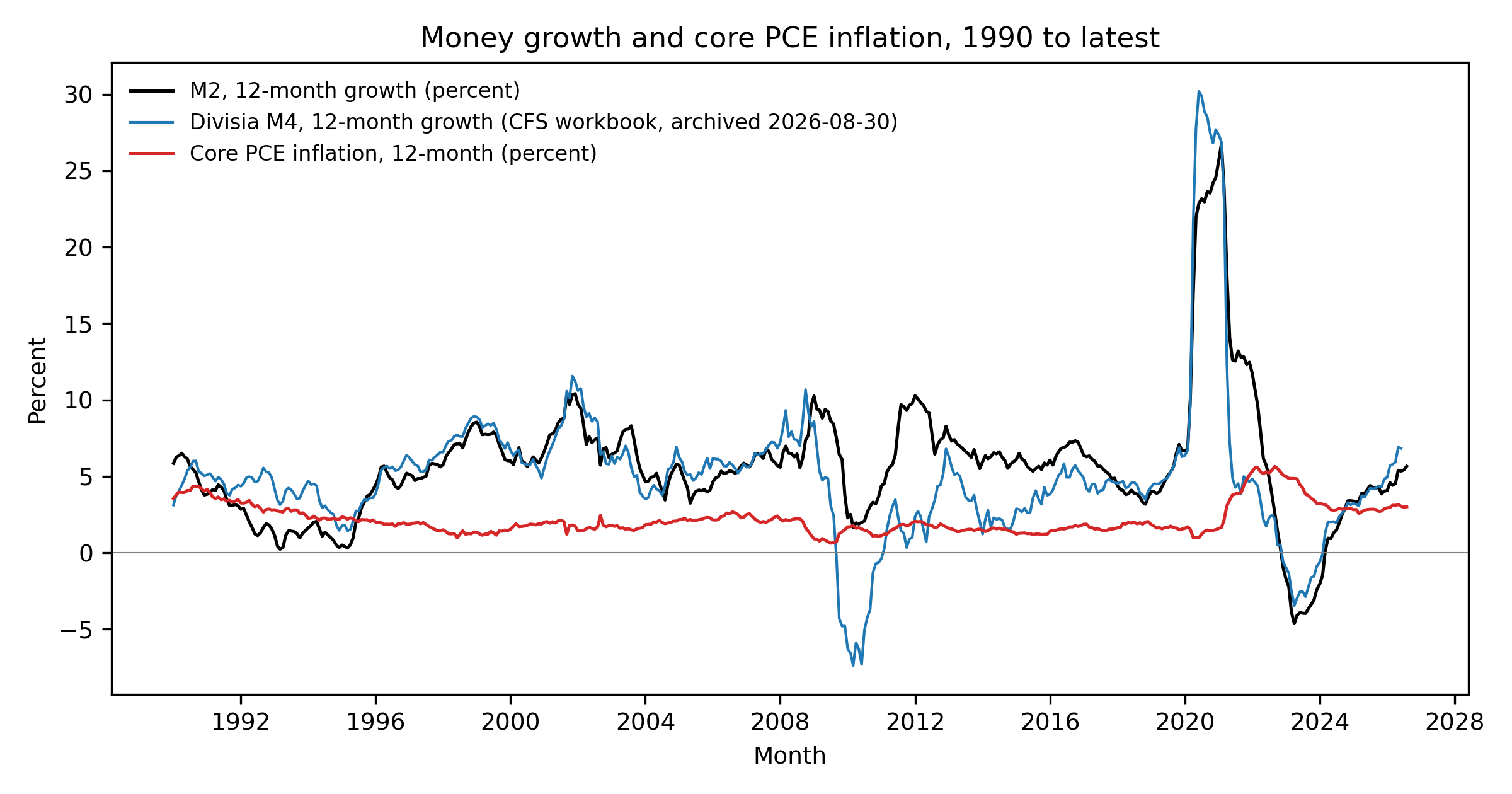
Cumulative growth from February 2020 to February 2022 was 40.2 percent for M2 and 32.7 percent for Divisia M4. Both aggregates contracted in 2023. For M2, the twelve-month growth rate turned negative in December 2022, the first negative reading in the M2SL series, which begins in January 1959, and stayed negative through February 2024. M2 velocity, defined as nominal GDP over M2, fell from 1.435 in the fourth quarter of 2019 to 1.126 in the second quarter of 2020 and had recovered to 1.418 by the second quarter of 2026. As of the latest data, twelve-month core PCE inflation was 3.0 percent in August 2026 and twelve-month DM4 growth was 6.8 percent in June 2026.
Two facts from Table 1 stand out. First, Divisia M4 peaked eight months earlier than M2. Divisia weights respond to the collapse in interest rates in March 2020, which raised the liquidity-service share of the broad aggregate’s components, and to the surge in Treasury bill issuance, which M2 does not include at all. Second, the lag from the M2 peak to the core inflation peak, nineteen months, is close to the “long and variable” lag of the monetarist tradition. This proximity makes the lead-lag chart persuasive, but it also makes the chart a weak test. The forecasting exercise below asks whether the lag was stable enough to use.
Figure 1 plots twelve-month growth in M2 and Divisia M4 against twelve-month core PCE inflation.
4. Methods
4.1 The forecasting problem
Let pi_t denote annualized monthly core PCE inflation, defined as 1,200 times the change in the log price index between month t minus 1 and month t. The forecast target at horizon h is average annualized inflation over the next h months,
pi(t, t+h) = (1,200 / h) × [log P(t+h) minus log P(t)].
Two horizons are examined, h = 12 and h = 24 months. Stock and Watson (1999) found Phillips curve models to be dominant at the twelve-month horizon. The twenty-four-month horizon is closer to the lag at which monetarists expect money growth to affect prices.
4.2 Benchmark model
The benchmark is a direct forecasting regression of the target on a constant, the twelve most recent monthly values of annualized core inflation, pi_t through pi_{t minus 11}, the current value of the GSCPI, and the current output gap. The GSCPI captures the supply-chain explanation of the 2021 inflation and the output gap captures the demand explanation. The benchmark specification is demanding, as it already contains the two variables emphasized by Bernanke and Blanchard (2023). Money growth improves the forecast only if it adds information beyond these variables. Two aspects of this benchmark specification warrant discussion. The output gap is a real-time series, constructed from the vintages available at each origin as described in Section 3.1, so the benchmark is one a forecaster could actually have run. Orphanides and van Norden (2002) show that real-time output gaps are heavily revised, and using the real-time series makes the benchmark weaker in absolute terms than the final-vintage benchmark of Appendix A; the comparison with the money-augmented challengers is correspondingly fairer, since every model now sees the same real-time information set apart from the Divisia series discussed in Section 3.3. The benchmark also contains no survey or market measures of inflation expectations, which many central bank models include. Adding them raises the bar for money further and would only strengthen a negative result, so the main text keeps the benchmark without them. Appendix B repeats the horse race with the University of Michigan Surveys of Consumers median expected inflation rate over the next twelve months added to the benchmark and to every challenger; the conclusions are unchanged.
4.3 Challenger models
Each linear challenger adds a single variable to the benchmark: twelve-month growth of a monetary aggregate at lag k, where k runs from 0 to 24 months. The maximum of 24 months is chosen for three reasons. It covers the eighteen-month lead of the retrospective chart with a margin of six months on either side, and it covers the two-to-three-year horizon at which Reynard (2007) and the monetarist tradition expect money growth to affect prices, since a twelve-month growth rate dated 24 months before the origin spans money growth from 36 to 24 months before the origin and, at the twenty-four-month horizon, up to 60 months before the end of the target window. Longer maximum lags would consume degrees of freedom in a minimum estimation window of 60 observations, and they would also leave the 2020 surge unused by the model until 2023 or later, which would remove from the evaluation the period in which the money signal is supposed to matter. At each forecast origin, the lag k is chosen by the Bayesian information criterion over the estimation window. This data-driven lag selection is used to provide a fair test. If money growth leads inflation by about eighteen months, as the retrospective chart suggests, the BIC should find that lag, or one close to it, and the forecasting model should benefit. Fixing the lag at one month would stack the deck against money; fixing it at eighteen months after observing the 2021 episode would stack the deck in its favor.
Four challenger series are used: M2 growth measured from final data, M2 growth measured from the real-time ALFRED vintage available at each origin, Divisia M4 growth, and Divisia M4 minus growth. The last two use final-vintage data for the reasons given in Section 3.3.
A fifth type of challenger tests the regime-dependence hypothesis directly. The threshold challenger adds two variables to the benchmark at the BIC-selected lag k: twelve-month money growth, and twelve-month money growth multiplied by an indicator equal to one when that growth exceeds 10 percent. The threshold was fixed at 10 percent before the models were run, as a round number that separates the ordinary range of post-1990 money growth from the 2020 to 2021 surge; it was not searched over. The specification lets the model learn a different slope for extreme readings, which a linear model cannot do. Threshold challengers are run for final-data M2 and for Divisia M4. One feature of the data limits the power of this test: between January 1985 and December 2019 twelve-month M2 growth exceeded 10 percent in only 6 months and Divisia M4 growth in 15, so at forecast origins before 2020 the threshold coefficient is estimated from very few observations. From January 2020 onward there were 24 such months for M2 and 13 for Divisia M4.
4.4 Estimation, evaluation, and tests
All models are estimated by ordinary least squares on an expanding window starting in January 1990, with a minimum of 60 observations before the first forecast is made. The data end in August 2026. Forecast origins run from January 2015 to August 2025 for h equal to 12, so that the last twelve-month target is the year ending August 2026, and from January 2015 to August 2024 for h equal to 24, so that the last twenty-four-month target also ends in August 2026. This gives 128 forecasts at the twelve-month horizon and 116 at the twenty-four-month horizon. Forecasts are direct: the model is estimated separately for each horizon and the forecast is the fitted value at the origin, so there is no iteration of a monthly model.
Accuracy is measured by root mean squared error (RMSE). The ratio of the challenger’s RMSE to the benchmark’s is reported, so that a ratio below one indicates the challenger is more accurate. Ratios are computed from unrounded RMSEs, so they may differ in the third decimal from the ratio of the rounded figures shown in the tables.
Two statistical tests are used to evaluate forecast accuracy. For a challenger that nests the benchmark, which is every money-augmented model compared with the benchmark, the appropriate test is the Clark and West (2007) adjusted statistic. The ordinary Diebold and Mariano (1995) test is biased against the larger model in that setting: under the null that money has no predictive content, the estimated coefficient on money adds noise to the challenger’s forecasts, so the challenger’s squared errors are larger even when the null is true. Clark and West correct for this by adding the squared difference between the two models’ forecasts back to the loss differential. The adjusted statistic is the t-ratio of the mean of the adjusted loss differential, computed with a Newey and West (1987) heteroskedasticity and autocorrelation consistent variance with a lag truncation of h minus 1, which is the appropriate correction when forecast errors overlap by h minus 1 periods. The test is one-sided: the alternative is that the challenger is more accurate, and the reported p-value is the probability, under the null, of a statistic at least as large as the one observed, computed from the standard normal distribution as Clark and West recommend. The sign convention is that a positive statistic favors the challenger and a negative statistic favors the benchmark; a negative statistic cannot reject the null however large it is in absolute value, because the test asks only whether the challenger is better.
For the comparison of two challengers with each other, Divisia M4 against real-time or final-data M2, and Divisia M4 against Divisia M4 minus, neither model nests the other, and the Diebold and Mariano (1995) test applies. It is the t-ratio of the mean difference in squared forecast errors, with the same Newey-West variance, and it is two-sided. By a convention used consistently in the tables and text, a positive statistic indicates that the first-named model, Divisia M4, has the smaller errors.
Results are also reported for two subsamples defined by the end date of the forecast target. The first contains targets ending before January 2020, which cover the low-inflation years: at the twelve-month horizon this is 48 forecasts with targets ending January 2016 to December 2019, and at the twenty-four-month horizon 36 forecasts with targets ending January 2017 to December 2019. The second contains targets ending January 2020 onward, through August 2026, which cover the pandemic, the inflation surge, and the disinflation: 80 forecasts at each horizon. The two subsamples add up to the full evaluation sample. The subsample results are reported as RMSEs and ratios only, without test statistics. With forecast errors overlapping by eleven or twenty-three months, the 36 to 80 forecasts in each subsample contain few independent observations, so formal tests would have low power and are not reported. To make the point concrete, the 36 twenty-four-month forecasts in the pre-2020 subsample have targets spanning January 2017 to December 2019, so the whole subsample covers only 36 months of outcomes, of which a single twenty-four-month forecast error occupies two thirds; the subsample contains, in effect, between one and two non-overlapping forecast errors.
A further caveat concerns inference after model selection. The lag of money growth in each challenger is chosen by the BIC at every origin, and the forecast evaluation then treats the selected model as if it had been specified in advance. Leeb and Pötscher (2005) show that the sampling distribution of estimates and test statistics after data-driven model selection can differ substantially from the distribution that applies to a fixed model, and that the difference does not vanish in large samples. In the present setting the effect most likely works against the challengers rather than for them, since selecting the lag at each origin from an expanding window adds estimation noise to the money models that the benchmark, whose specification is fixed, does not carry. The Clark-West and Diebold-Mariano statistics reported below should be read with that in mind: they describe the accuracy of the selection-plus-forecasting procedure a practitioner would actually have followed, not the accuracy of a known best lag.
4.5 The P-star price gap
The P-star framework of Hallman, Porter, and Small (1991) is estimated quarterly. The price level P is the GDP deflator, computed as nominal over real GDP times 100. Velocity V is nominal GDP over the quarterly average of the monetary aggregate. The log of equilibrium velocity, log(V-star), is defined as the trend of log velocity. The equilibrium price level is
P-star = M × exp(log V-star) / potential GDP × 100,
and the price gap is 100 times the log difference between the actual and equilibrium price levels. A negative gap means the actual price level is below the level implied by the money stock, trend velocity, and potential output, which the framework interprets as a signal of future inflation.
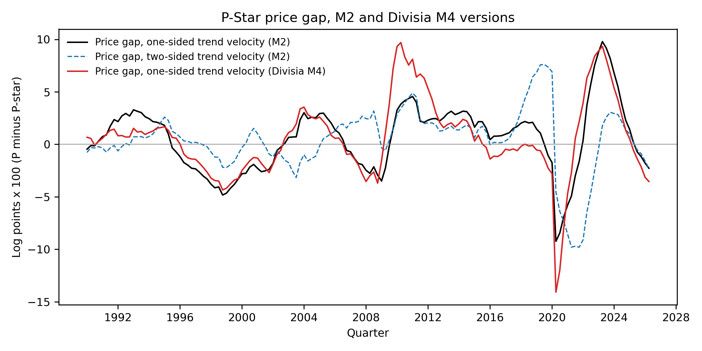
Three versions of the velocity trend are computed. The one-sided recursive version re-estimates a Hodrick and Prescott (1997) trend, with the conventional quarterly smoothing parameter of 1,600, at each quarter using only data up to that quarter, with a minimum of twenty observations. This is the version a real-time forecaster could have used and is the primary specification in this paper. The two-sided version applies the same filter to the full sample and is the version most commonly reported; it uses information from after each quarter and is therefore not a real-time object. As a robustness check on the choice of filter, a third version fits a linear time trend to log velocity recursively, again using only data up to each quarter. The one-sided and two-sided HP versions differ most at the end of the sample and around turning points, coinciding with the 2020 episode.
The forecasting regression follows the original paper: the change in inflation over the next four quarters, defined as inflation over the following four quarters minus inflation over the trailing four quarters, is regressed on a constant, the current price gap, and current quarterly inflation. The full set of coefficients is reported because the coefficient on current inflation is of interest and its inclusion affects the significance of the gap; results for a version that omits current inflation are also reported. Standard errors are HAC with four lags. The sample is 1990Q1 to 2025Q2, 142 quarters; it ends in 2025Q2 rather than 2026Q2 because the dependent variable is inflation over the following four quarters, so the last observation whose outcome is known by 2026Q2 is dated 2025Q2.
4.6 Use of computational tools
All computations were performed in Python scripts included in the replication package. A language model was used for drafting and editing assistance. The author verified every number and interpretation.
5. Results
5.1 Twelve-month horizon
Table 2 reports the horse race at the twelve-month horizon.
| Sample and model | n | RMSE | Ratio to benchmark | CW statistic | One-sided p-value |
|---|---|---|---|---|---|
| Full sample | |||||
| Benchmark | 128 | 1.185 | 1.000 | ||
| plus M2 growth (final data) | 128 | 1.271 | 1.073 | minus 0.78 | 0.783 |
| plus M2 growth (real-time data) | 128 | 1.258 | 1.062 | minus 0.42 | 0.663 |
| plus Divisia M4 growth | 128 | 1.234 | 1.041 | minus 1.69 | 0.955 |
| plus Divisia M4 minus growth | 128 | 1.296 | 1.094 | minus 2.40 | 0.992 |
| Targets ending before January 2020 (descriptive) | |||||
| Benchmark | 48 | 0.201 | 1.000 | ||
| plus M2 growth (final data) | 48 | 0.229 | 1.139 | ||
| plus M2 growth (real-time data) | 48 | 0.234 | 1.160 | ||
| plus Divisia M4 growth | 48 | 0.218 | 1.083 | ||
| plus Divisia M4 minus growth | 48 | 0.210 | 1.042 | ||
| Targets ending January 2020 onward (descriptive) | |||||
| Benchmark | 80 | 1.490 | 1.000 | ||
| plus M2 growth (final data) | 80 | 1.598 | 1.072 | ||
| plus M2 growth (real-time data) | 80 | 1.580 | 1.060 | ||
| plus Divisia M4 growth | 80 | 1.551 | 1.041 | ||
| plus Divisia M4 minus growth | 80 | 1.631 | 1.095 |
Notes: RMSE in percentage points of annualized inflation. Ratios are computed from unrounded RMSEs. CW is the Clark and West (2007) adjusted statistic for nested models against the benchmark, with Newey-West variance and lag truncation 11; the test is one-sided against the alternative that the challenger is more accurate, so a positive statistic favors the challenger and a negative statistic favors the benchmark. Subsample rows are descriptive; no test statistics are reported for them because the effective number of independent observations is small (Section 4.4). The benchmark uses the real-time output gap described in Section 3.1; Appendix A reports the same table with the final-vintage gap.
No challenger beats the benchmark, and every challenger actively worsens it. Adding M2 growth raises the RMSE by 7.3 percent with final data and 6.2 percent with real-time data over the full sample. The Clark-West statistics are negative, so the adjusted comparison, which gives the challenger credit for the noise introduced by estimating a coefficient on money, still points toward the benchmark, and the test does not find that either M2 model is significantly more accurate than the benchmark. In the pre-2020 subsample the deterioration from adding M2 is larger in proportional terms, 14 to 16 percent: during the decade of steady 6 to 7 percent M2 growth and below-target inflation, a model that leaned on money systematically overpredicted. In the subsample of targets ending 2020 onward the benchmark’s RMSE rises more than sevenfold, to 1.49 percentage points, because every model missed the size of the surge, and adding M2 raises it by a further 6.0 to 7.2 percent.
The Divisia aggregates do not help at this horizon either. Divisia M4 raises the RMSE by 4.1 percent and Divisia M4 minus by 9.4 percent, and the negative Clark-West statistics for both indicate their forecasts were less accurate than the benchmark’s, even after the nesting adjustment. The same pattern appears in both subsamples. The direct comparison of Divisia M4 with M2, reported in Section 5.4, finds no significant difference between them at this horizon.
The finding that money growth does not improve forecast accuracy at the twelve-month horizon, in a sample that includes the 2021 episode, is consistent with Stock and Watson (1999).
5.2 Twenty-four-month horizon
Table 3 reports the twenty-four-month horizon, which is where the monetarist case should be strongest.
| Sample and model | n | RMSE | Ratio to benchmark | CW statistic | One-sided p-value |
|---|---|---|---|---|---|
| Full sample | |||||
| Benchmark | 116 | 1.438 | 1.000 | ||
| plus M2 growth (final data) | 116 | 1.665 | 1.158 | minus 2.18 | 0.985 |
| plus M2 growth (real-time data) | 116 | 1.648 | 1.146 | minus 2.21 | 0.987 |
| plus Divisia M4 growth | 116 | 1.465 | 1.018 | minus 0.73 | 0.768 |
| plus Divisia M4 minus growth | 116 | 1.574 | 1.094 | minus 1.45 | 0.927 |
| Targets ending before January 2020 (descriptive) | |||||
| Benchmark | 36 | 0.069 | 1.000 | ||
| plus M2 growth (final data) | 36 | 0.088 | 1.272 | ||
| plus M2 growth (real-time data) | 36 | 0.104 | 1.505 | ||
| plus Divisia M4 growth | 36 | 0.109 | 1.570 | ||
| plus Divisia M4 minus growth | 36 | 0.085 | 1.229 | ||
| Targets ending January 2020 onward (descriptive) | |||||
| Benchmark | 80 | 1.731 | 1.000 | ||
| plus M2 growth (final data) | 80 | 2.004 | 1.158 | ||
| plus M2 growth (real-time data) | 80 | 1.983 | 1.145 | ||
| plus Divisia M4 growth | 80 | 1.762 | 1.018 | ||
| plus Divisia M4 minus growth | 80 | 1.894 | 1.094 |
Notes: As for Table 2, with Newey-West lag truncation 23.
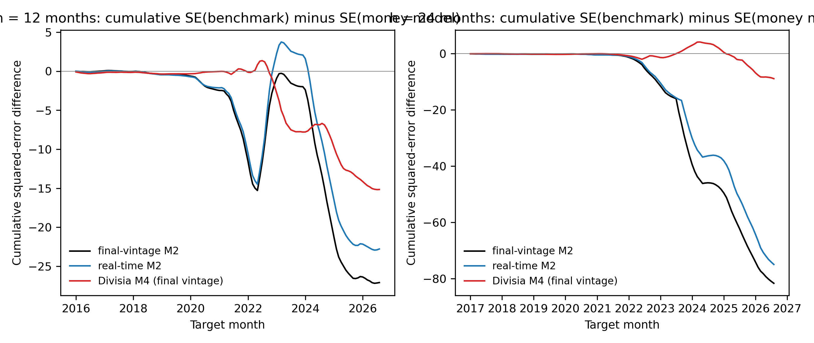
Two findings emerge from the results for the twenty-four-month horizon. First, M2 does worse, not better, at the longer horizon. Adding M2 growth raises the RMSE by 15.8 percent with final data and 14.6 percent with real-time data over the full sample, and by 14 to 16 percent in the subsample of targets ending 2020 onward. The Clark-West statistics are about minus 2.2 for both M2 models, which means that even after the adjustment for nesting, the money-augmented forecasts were further from the outcome than the benchmark’s by a margin that is large relative to its sampling variability. The one-sided test cannot, by construction, declare the benchmark significantly better; what it says is that there is no evidence at all that M2 helped, and the point estimates say it actively hurt. This is the opposite of what the lead-lag chart implies. The reason, examined in Section 5.3 and Section 6, is that the BIC chose the maximum allowed lag of 24 months for M2 at more than half of the forecast origins (Table 4). The model was therefore usually reading M2 growth from two years earlier, which in 2022 and 2023 meant the 2020 and 2021 surge, and in 2024 and 2025 meant the 2022 and 2023 contraction. Money growth was pointing the model toward continued high inflation when inflation was already falling, and toward deflation when inflation had stabilized near 3 percent.
Second, Divisia M4 behaves differently from M2 at this horizon. Its RMSE ratio is 1.018 over the full sample and 1.018 in the 2020 onward subsample, and its Clark-West statistic of minus 0.73 is much closer to zero than the M2 statistics. Divisia M4 minus, which excludes Treasury bills, lies between the two. Divisia M4 does not improve on the benchmark, but it impairs forecast accuracy less than M2 does, and Section 5.4 shows that the difference between the two aggregates is statistically significant at the 5 percent level, though only marginally so in the like-for-like final-vintage comparison. The ordering predicted by aggregation theory, Divisia better than simple sum, therefore appears in the data, but with two qualifications that recur throughout the paper. First, ‘better’ here means ‘not much worse than a benchmark without money’ rather than ‘better than the benchmark,’ and second, the Divisia series is final vintage while the fairest M2 comparison is the real-time one. The difference between Divisia M4 and Divisia M4 minus, by contrast, is not statistically significant: a Diebold-Mariano test of the two gives a statistic of 1.46 (two-sided p-value 0.143) at twelve months and 1.57 (p-value 0.116) at twenty-four months, so the paper does not claim that excluding Treasury bills makes a detectable difference.
Figure 2 plots the cumulative difference in squared forecast errors between each challenger and the real-time benchmark at the twenty-four-month horizon. A rising line means the challenger is accumulating larger errors. The M2 lines rise steeply from 2022 onward; the Divisia M4 line stays close to zero.
5.3 Instability of the selected lag
Table 4 summarizes, for each challenger and horizon, the lag of twelve-month money growth chosen by the Bayesian information criterion across the forecast origins (128 origins at twelve months, 116 at twenty-four months; lags from 0 to 24 were allowed). The table is placed directly after the horse race because the instability it documents is the main mechanism behind the poor performance of the money models, and the remaining sections refer back to it.
| Horizon and challenger | Mean lag | Median lag | Standard deviation | Share of origins choosing lag 24 | Share of origins choosing lag 0 |
|---|---|---|---|---|---|
| months, M2 (final data) | 6.8 | 9 | 6.8 | 0.09 | 0.16 |
| 12 months, M2 (real-time data) | 5.2 | 4 | 6.8 | 0.09 | 0.40 |
| 12 months, Divisia M4 | 12.5 | 9 | 10.0 | 0.41 | 0.05 |
| 12 months, Divisia M4 minus | 6.8 | 9 | 5.0 | 0.04 | 0.08 |
| 12 months, M2 threshold | 4.8 | 5 | 6.0 | 0.08 | 0.09 |
| 12 months, Divisia M4 threshold | 13.5 | 17 | 10.8 | 0.50 | 0.09 |
| 24 months, M2 (final data) | 13.4 | 24 | 11.6 | 0.53 | 0.38 |
| 24 months, M2 (real-time data) | 13.7 | 24 | 11.6 | 0.55 | 0.38 |
| 24 months, Divisia M4 | 17.1 | 24 | 10.7 | 0.71 | 0.15 |
| 24 months, Divisia M4 minus | 12.8 | 6.5 | 11.1 | 0.49 | 0.10 |
| 24 months, M2 threshold | 6.0 | 0 | 10.1 | 0.23 | 0.69 |
| 24 months, Divisia M4 threshold | 18.1 | 24 | 10.2 | 0.75 | 0.11 |
Notes: Lags in months. The threshold challengers are those of Table 7.
The selected lags show two patterns. At the twenty-four-month horizon the criterion pushed the linear challengers toward the longest lag allowed at between half and three quarters of origins, while also choosing lag 0 at more than a third of origins for the M2 models, so the selected lag jumped between the two ends of the allowed range rather than settling near the eighteen months that the lead-lag chart suggests. At the twelve-month horizon the M2 lags are short and dispersed, with lag 0 chosen at 40 percent of origins for real-time M2. Neither pattern is what one would expect if money growth led inflation by a stable interval, and a model that is alternately reading money growth from two years ago and from the current month cannot produce a stable forecast.
The bimodal pattern at twenty-four months has a mechanical reading, and the sequence of selected lags across origins shows it. For final-data M2 the criterion chose lag 24 at almost every origin from mid-2017 to mid-2021, when the estimation window ended before the surge or contained it only as a regressor dated two years back; the pre-2020 sample contains no stable intermediate lag, so the criterion settled at the boundary of the allowed range. From mid-2022 onward, which is the first point at which the surge months of 2020 and 2021 enter the window as origins with completed twenty-four-month targets, the criterion switched to lag 0 and stayed there through the end of the sample. At that point the contemporaneous reading, which aligns the surge directly with the inflation that followed it, fit better than any lag between 1 and 23 months, because the intermediate lags align the surge with only part of the inflation and the preceding decade supplies no information to pull the choice toward an intermediate value. The criterion therefore alternated between the two ends of the range because the sample contains no stable intermediate lag, not because it found one and lost it. The median lag of 0 for the M2 threshold model at twenty-four months, with lag 0 chosen at 69 percent of origins against 38 percent for the linear M2 models, fits the same reading. With a threshold term in the model, the months in which money growth exceeded 10 percent carry the fit by themselves: at lag 0 the indicator switches on during the surge months and the threshold coefficient absorbs the inflation that followed, so the long lag that the linear model used before 2022 is unnecessary, and the threshold model chose lag 0 at most origins before 2020 as well as after 2022. The threshold model abandons the long lag because the indicator does the alignment for it, which is also why its errors fall relative to the linear model without falling below the benchmark (Table 7). Section 6.1 draws out the consequence for the lead-lag chart.
5.4 Divisia M4 against M2 directly
Table 5 reports the direct comparison of the Divisia M4 model with the M2 model, using both the real-time M2 model, which is the fairest comparison from the forecaster’s point of view, and the final-data M2 model. Neither model nests the other, so the Diebold-Mariano test applies.
| Horizon | M2 model | n | RMSE, plus M2 | RMSE, plus Divisia M4 | DM statistic | Two-sided p-value |
|---|---|---|---|---|---|---|
| months | real-time data | 128 | 1.258 | 1.234 | 0.30 | 0.768 |
| 12 months | final data | 128 | 1.271 | 1.234 | 0.49 | 0.621 |
| 24 months | real-time data | 116 | 1.648 | 1.465 | 2.13 | 0.033 |
| 24 months | final data | 116 | 1.665 | 1.465 | 2.00 | 0.045 |
Notes: Diebold and Mariano (1995) test of equal squared-error loss with Newey-West variance, lag truncation h minus 1. A positive statistic means the Divisia M4 model has the smaller errors. All models contain the real-time output gap benchmark, and the RMSEs are those reported in Tables 2 and 3.
At twelve months the two aggregates are indistinguishable. At twenty-four months the Divisia M4 model’s errors are smaller than the M2 model’s at the 5 percent level, with a p-value of 0.033 against the real-time M2 model and 0.045 against the final-data M2 model. The first of these comparisons sets a final-vintage Divisia series against a real-time M2 series, so part of the gap may reflect vintage rather than aggregation; the second, which compares final vintage with final vintage, is the like-for-like comparison, and it is only marginally significant; with survey expectations added to the benchmark (Appendix B) its p-value rises to 0.057. The choice of monetary aggregate makes a statistically detectable difference only in this comparison and in the results shown in Table 3, and the difference is between two models that both fail to beat the benchmark (Table 6).
5.5 Real-time versus final M2
A natural objection to any negative finding about money is that the money data have been revised. Table 6 shows that this is not the explanation.
| Horizon | M2, final data | M2, real-time ALFRED vintages | Divisia M4, final data |
|---|---|---|---|
| months | 1.073 | 1.062 | 1.041 |
| 24 months | 1.158 | 1.146 | 1.018 |
Notes: Ratios computed from unrounded RMSEs against the real-time output gap benchmark. The Divisia M4 column is final vintage; see Section 3.3.
The real-time M2 model is marginally more accurate than the final-data M2 model at both horizons, by approximately 0.01 in the ratio. Appendix A shows that the same ratios computed against the final-vintage output gap benchmark are 1.057, 1.048, and 1.046 at twelve months and 1.148, 1.138, and 1.024 at twenty-four months, so moving to the real-time benchmark raises the M2 ratios slightly and lowers the Divisia M4 ratios slightly without changing any conclusion. While this difference implies that real-time forecast errors were slightly smaller than the final data suggest, it is not large enough to change the conclusion. Since M2 revisions are modest, the forecast errors appear to reflect an unstable relationship between money and inflation rather than inaccuracies in the monetary data.
5.6 A threshold specification
If the money-inflation link is strong only when money growth is extreme, a model that allows a separate slope above a threshold should do better than the linear money models, and if the hypothesis is right in a strong form it should also beat the benchmark. Table 7 reports the threshold challengers described in Section 4.3.
| Horizon and aggregate | RMSE | Ratio to benchmark | Ratio to linear money model | CW against benchmark (p) | CW against linear money model (p) | Ratio to benchmark, targets before 2020 | Ratio to benchmark, targets 2020 onward | Median BIC lag |
|---|---|---|---|---|---|---|---|---|
| months, M2 (final) | 1.220 | 1.030 | 0.960 | 0.25 (0.402) | 1.17 (0.122) | 1.164 | 1.029 | 5 |
| 12 months, Divisia M4 | 1.251 | 1.056 | 1.014 | minus 0.55 (0.710) | 0.03 (0.488) | 1.074 | 1.056 | 17 |
| 24 months, M2 (final) | 1.535 | 1.067 | 0.922 | minus 1.08 (0.861) | 1.48 (0.070) | 1.231 | 1.067 | 0 |
| 24 months, Divisia M4 | 1.417 | 0.985 | 0.967 | 1.16 (0.124) | 1.04 (0.149) | 1.497 | 0.985 | 24 |
Notes: Each threshold model adds to the benchmark both twelve-month money growth and money growth multiplied by an indicator for growth above 10 percent, at the same BIC-selected lag. Full-sample n is 128 at twelve months and 116 at twenty-four months. CW statistics are Clark and West (2007) one-sided tests with one-sided p-values in parentheses; the threshold model nests both the benchmark and the corresponding linear money model. Subsample ratios are descriptive. All models contain the real-time output gap benchmark; Appendix A reports the final-vintage version.
The threshold specification was estimated as a direct test of the regime-dependence hypothesis, and the test is inconclusive because of low statistical power. Relative to the corresponding linear model, the threshold version lowers the RMSE in three of the four cases, by between 3.3 and 7.8 percent, and raises it by 1.4 percent in the fourth, Divisia M4 at twelve months; the Clark-West tests against the linear model have one-sided p-values between 0.070 and 0.488, suggestive at best and never significant at the 5 percent level. Relative to the benchmark, three of the four threshold models still have ratios above one. The exception is Divisia M4 at twenty-four months, whose ratio of 0.985 is the only ratio below one in Table 7; its Clark-West statistic against the benchmark is 1.16 with a p-value of 0.124, so the improvement is not statistically distinguishable from zero. In the pre-2020 subsample the threshold models are as bad as the linear ones, which is expected, since the threshold coefficient could not be estimated from the handful of pre-2020 months above 10 percent. Two things should be said about this result. First, the hypothesis remains plausible: the point estimates move in the predicted direction in three of four cases. Second, the test has low power, since the threshold coefficient is identified by the few months of money growth above 10 percent in 2020 and 2021 and is evaluated over overlapping forecast errors, and a p-value of 0.124 in the one favorable case is what a true but modest effect would often produce in a sample of this size. The evidence therefore neither supports nor rejects regime dependence; the test is inconclusive and the hypothesis is left open.
5.7 The P-star price gap
Table 8 reports the P-star regressions over 1990Q1 to 2025Q2, leading with the one-sided recursive trend that a real-time user could have computed.
| Aggregate and trend | Constant (SE) | Gap coefficient (SE) | Gap p-value | Current inflation coefficient (SE) | Current inflation p-value | R-squared | Gap coefficient without current inflation (SE) | p-value | R-squared |
|---|---|---|---|---|---|---|---|---|---|
| M2, one-sided recursive HP | 0.347 (0.283) | minus 0.156 (0.079) | 0.047 | minus 0.117 (0.148) | 0.431 | 0.227 | minus 0.163 (0.073) | 0.026 | 0.207 |
| M2, two-sided HP | 0.914 (0.291) | minus 0.199 (0.079) | 0.012 | minus 0.373 (0.131) | 0.004 | 0.254 | minus 0.117 (0.094) | 0.214 | 0.095 |
| M2, recursive linear trend | 0.279 (0.336) | minus 0.020 (0.018) | 0.257 | minus 0.214 (0.144) | 0.137 | 0.098 | minus 0.015 (0.020) | 0.449 | 0.034 |
| Divisia M4, one-sided recursive HP | 0.280 (0.307) | minus 0.119 (0.079) | 0.132 | minus 0.096 (0.170) | 0.572 | 0.177 | minus 0.127 (0.074) | 0.084 | 0.164 |
| Divisia M4, two-sided HP | 0.717 (0.310) | minus 0.180 (0.072) | 0.013 | minus 0.285 (0.141) | 0.043 | 0.288 | minus 0.147 (0.074) | 0.048 | 0.177 |
| Divisia M4, recursive linear trend | minus 0.361 (0.565) | minus 0.068 (0.041) | 0.100 | minus 0.253 (0.145) | 0.082 | 0.187 | minus 0.054 (0.042) | 0.201 | 0.099 |
Notes: Dependent variable is inflation over the following four quarters minus inflation over the trailing four quarters, in percentage points. n equals 142 in every regression. Standard errors are HAC with four lags; p-values are two-sided. The last three columns report the regression of the same dependent variable on a constant and the gap alone.
The overall P-star evidence is not robust: the sign of the gap is stable, but its significance depends on the aggregate and on the trend method, and no specification is significant in every form. Against that background there is one exception. With the one-sided recursive trend, which is the only version available in real time, the M2 gap has the expected negative sign and is significant at the 5 percent level, with a p-value of 0.047; current inflation adds nothing in that regression, and dropping it moves the gap’s p-value to 0.026 with a small loss of fit, the R-squared falling from 0.227 to 0.207. This is the one piece of evidence in the paper that broad money carried usable quantitative information in real time, and it is a fragile exception rather than a general finding, for two reasons. First, the result depends on the aggregate: the one-sided Divisia M4 gap is not significant at the 5 percent level in either form, with p-values of 0.132 and 0.084. Second, it depends on the trend method. With the two-sided trend, which uses information from after each quarter, both gaps are significant at the 5 percent level in the full specification and the fit improves to R-squared values of 0.25 to 0.29, though for M2 the two-sided gap loses its significance when current inflation is dropped. The recursive linear trend performs poorly: the gap coefficients shrink toward zero and are insignificant, because a recursive linear trend adapts too slowly to the sharp collapse in velocity that occurred in 2020Q2, so the implied gap is implausibly large, reaching minus 40 percent for M2 and minus 28 percent for Divisia M4 at the end of 2021 and still minus 13 and minus 9 percent in 2026Q2. Orphanides and van Norden (2002) document the same problem for real-time output gaps: the end-of-sample estimate of a trend is its least reliable part, and a trend estimated recursively, without the benefit of later data, can misread a structural break as a temporary gap for years. The P-star result therefore depends on the HP filter doing a reasonable job of tracking trend velocity, and the overall evidence is sensitive to both the aggregate and the trend method: a marginal real-time result for M2 and a null result for Divisia M4.
The gap series plotted in Figure 3 show the large movements that occurred in 2020. The one-sided M2 gap fell to minus 9.2 percent in 2020Q2 and the one-sided Divisia M4 gap to minus 14.1 percent, the widest readings in the sample, implying in the P-star framework that the price level was far below what the money stock implied. Both had largely closed by the end of 2021 in the one-sided reading: the M2 gap was minus 1.6 percent in 2021Q4 and the Divisia gap had turned positive at 2.2 percent. The two-sided gaps, which use information from after each quarter, yield different results: the M2 gap reached its minimum of minus 9.8 percent in 2021Q4 and the Divisia gap was still at minus 7.4 percent in that quarter. The two readings for the end of 2021 have different implications: the one-sided gap suggests the inflationary impulse had been absorbed, while the two-sided gap suggests it was only beginning. A real-time user had only the first. As of 2026Q2 the HP-based gaps are modestly negative, minus 2.3 percent for M2 and minus 3.5 percent for Divisia M4 in both versions.
6. Discussion
6.1 Why the lead-lag chart misleads
The chart of M2 growth leading inflation by eighteen months is correct as a description of 2020 to 2022 and misleading as evidence about forecasting. Three features of the forecasting results explain this discrepancy.
First, the relationship did not hold in the preceding decade. In the pre-2020 subsample, adding M2 growth to the benchmark raised the RMSE by 14 to 16 percent at twelve months and by 27 to 51 percent at twenty-four months. These are descriptive ratios on small samples, and they rest on very small benchmark RMSEs of 0.20 and 0.07 percentage points, so modest absolute differences appear as large ratios; their direction, however, is unambiguous. A forecaster who had adopted a money-augmented model in 2015 would have spent five years overpredicting inflation and would have had every reason to abandon it before 2020.
Second, the lag is not stable. Table 4 in Section 5.3 reports the distribution of BIC-selected lags. At the twelve-month horizon the BIC chose lags for final-data M2 anywhere between 0 and 24 months, with a mean of 7 and a median of 9, and chose lag 0 at 16 percent of origins and lag 24 at 9 percent. At the twenty-four-month horizon it chose 24 months, the maximum allowed, at 53 percent of origins, with a median of 24. The chart’s eighteen-month lag is one draw from a wide distribution, and a model using a long lag performed poorly in 2023 to 2025 because it was still reacting to the 2020 to 2021 surge after inflation had turned.
Third, the information in money growth in 2020 was a level shift, not a signal within the normal range. In the M2SL series from 1959 to 2019, twelve-month M2 growth never exceeded 13.8 percent (its peak was in February 1976) and from 1990 to 2019 it stayed between 0.2 and 10.4 percent; from May 2020 to March 2021 it was above 20 percent for eleven consecutive months. A linear regression estimated over three decades in which money growth varied between 0 and 10 percent has no basis for predicting what a 27 percent reading means. The coefficient it has learned is small, because over most of the sample money growth did not forecast inflation, and so the model treats the surge as a modest signal rather than the regime break it may have been. This is the natural time-series counterpart of the cross-country pattern in Borio, Hofmann, and Zakrajšek (2023), in which the money-inflation link is strong when money growth is extreme and weak when it is ordinary. The threshold results in Section 5.6 directly test this hypothesis, and the test is inconclusive because of low statistical power. Allowing a separate slope above 10 percent improves the money models by a few percent in three of four cases, but not significantly, and only one of four threshold models has an RMSE below the benchmark, by an amount indistinguishable from zero. Regime dependence remains the most plausible account of why the lead-lag chart looks the way it does, and the test has too little power, with the threshold identified by a handful of months, either to confirm or to reject it; on the evidence here it is an open hypothesis, not a finding. One reason the test is weak is mechanical: a model can learn about the effects of extreme money growth only from such episodes, and before 2020 the United States sample contained almost none.
6.2 What Divisia M4 adds
Divisia M4 differs from M2 in two respects. Its growth peaked in June 2020, eight months before M2 and twenty-seven months before core inflation peaked, because the Divisia weights respond to the collapse in interest rates and because the aggregate includes the surge in Treasury bill issuance. And at the twenty-four-month horizon its forecast errors are smaller than those of the M2 model, with a p-value of 0.033 against real-time M2 and a marginal 0.045 against final-vintage M2, while neither improves on the benchmark.
This is a qualified and partial result for aggregation theory. Barnett (1980) argued that simple-sum aggregates mismeasure money and that the mismeasurement would be largest during periods of sharp interest rate movements, such as March 2020, since that is when the liquidity-service weights change most. The Divisia aggregate tracked the 2020 shock earlier and gave less misleading signals in its aftermath. The result is qualified in two ways. Divisia M4 did not beat a benchmark that contains no money at all. And the Divisia series used here is the final vintage, whereas the strictest M2 comparison uses real-time vintages. The archived copies suggest Divisia revisions are small, but the direction of the vintage effect is known from the M2 results: the real-time M2 model is marginally more accurate than the final-vintage M2 model, so vintage effects are not large in this sample, and a real-time Divisia series would be expected to change the comparison with M2 by a similarly small amount in either direction. The comparison that holds vintage constant, final-vintage Divisia M4 against final-vintage M2, is significant only at the margin, with a p-value of 0.045. The evidence therefore supports a modest statement: in final-vintage data over this sample, the Divisia M4 model made smaller errors than the M2 model at the twenty-four-month horizon, and the difference is at the edge of what the sample can detect.
6.3 Directional versus quantitative information
The results suggest a distinction that the money-inflation debate often blurs. Money growth in 2020 carried directional information. The unprecedented expansion of the quantity of money, visible in Divisia form by mid-2020, signaled an inflation risk that the Phillips curve and the supply-chain index did not capture. That is consistent with the Greenwood and Hanke (2021) argument and with the cross-country evidence of Borio, Hofmann, and Zakrajšek (2023). A claim of directional information should be confronted with the data rather than asserted, so Table 9 reports a structured descriptive exercise: a probit regression in which the dependent variable equals one in the months when the benchmark’s absolute forecast error exceeded its own full-sample RMSE, and the explanatory variable is twelve-month money growth at the forecast origin, or twelve months before it.
| Horizon | Regressor | n | Events | Coefficient | HAC standard error | p-value | Pseudo R-squared |
|---|---|---|---|---|---|---|---|
| months | M2 growth, real-time data, at origin | 128 | 23 | 0.240 | 0.108 | 0.026 | 0.64 |
| 12 months | M2 growth, final data, at origin | 128 | 23 | 0.247 | 0.117 | 0.036 | 0.65 |
| 12 months | Divisia M4 growth, at origin | 128 | 23 | 0.163 | 0.046 | 0.000 | 0.42 |
| 12 months | M2 growth, real-time data, twelve months earlier | 128 | 23 | 0.081 | 0.031 | 0.010 | 0.16 |
| 12 months | Divisia M4 growth, twelve months earlier | 128 | 23 | 0.114 | 0.028 | 0.000 | 0.33 |
| 24 months | M2 growth, real-time data, at origin | 116 | 33 | 0.124 | 0.064 | 0.052 | 0.30 |
| 24 months | M2 growth, final data, at origin | 116 | 33 | 0.124 | 0.065 | 0.057 | 0.29 |
| 24 months | Divisia M4 growth, at origin | 116 | 33 | 0.105 | 0.044 | 0.016 | 0.22 |
| 24 months | M2 growth, real-time data, twelve months earlier | 116 | 33 | 0.089 | 0.024 | 0.000 | 0.15 |
| 24 months | Divisia M4 growth, twelve months earlier | 116 | 33 | 0.218 | 0.139 | 0.116 | 0.32 |
Notes: The dependent variable equals one when the absolute forecast error of the real-time benchmark exceeds the benchmark’s full-sample RMSE (1.185 percentage points at twelve months, 1.438 at twenty-four months) and zero otherwise. Money growth is twelve-month growth in percent. Standard errors are HAC; p-values are two-sided, and 0.000 denotes a value below 0.0005. The events form two contiguous runs at twelve months (April 2020 to August 2023) and three at twenty-four months (December 2019 to August 2023), so the effective number of independent observations is far smaller than n.
Money growth at the origin predicts the benchmark’s large errors at the twelve-month horizon for both aggregates, and at the twenty-four-month horizon for Divisia M4 and marginally for M2, with p-values of 0.052 and 0.057; the lagged readings do so as well, except for Divisia M4 at twenty-four months. The caveat is severe. Because the large errors fall in two or three contiguous runs, the 23 and 33 events are far fewer independent observations than they appear, and the HAC standard errors can correct for this only in part. The high pseudo R-squared values for the at-origin regressors at twelve months, 0.64 and 0.65 for M2, are most likely an artifact of this clustering: a single regressor that is elevated during one contiguous run of events and low elsewhere separates the two classes almost perfectly, which inflates the fit without adding independent evidence. The probit is therefore a structured description of the coincidence between extreme money growth and the benchmark’s failures, not a test of the directional claim, and I report it as such. But money growth did not carry stable quantitative information of the kind a forecasting regression can use. Its coefficient, its lag, and its relevance all appear to have changed with the regime, and the one specification in this paper that tries to capture the change, the threshold model, lacks the power to settle whether it does.
The practical implication, stated with the modesty the evidence requires, is that monetary aggregates do not belong in the forecasting equation but may belong on the forecaster’s watch list. The probit results suggest that extreme readings of broad money, particularly in Divisia form, were associated with the episodes in which a standard model was about to fail; a forecaster who monitored them would have had a reason to consider scenarios outside the model’s range. That is a weaker claim than the monetarist tradition makes and a stronger one than a model with no money at all implies, and this paper cannot establish more than that.
6.4 The P-star evidence
The P-star results fit the same pattern. The evidence is not robust: the one-sided Divisia M4 gap is insignificant, the two-sided trend that makes both gaps significant is not available in real time, and the recursive linear trend removes every result, so the findings are sensitive to both the aggregate and the trend method. The one exception is the real-time, one-sided M2 gap, which is significant at the 5 percent level with a p-value of 0.047; given the pattern around it, I treat it as fragile. Over the full sample from 1990 the price gap does have the right sign for both aggregates and every trend specification. And at the end of 2021 the one-sided gap had closed, indicating that the impulse had passed, while the two-sided gap, constructed with knowledge of 2022 and 2023, still showed a large overhang. Although the P-star framework correctly assumes that an excess of money relative to trend velocity and potential output predicts inflation, it failed to provide a usable real-time signal for the same reason Orphanides and van Norden (2002) identified for the output gap: end-of-sample trend estimation is unreliable when the sample ends in an unusual quarter. Similarly, the recursive linear trend failed because it was too rigid to follow the 2020 collapse in velocity, producing gaps so large that they were uninformative. This is the velocity counterpart of the real-time trend uncertainty that Orphanides and van Norden (2002) document for the output gap: a trend estimated with only the data available at the time is least reliable exactly when the economy has just moved, which is when a price gap would be most useful.
7. Limitations
Several limitations qualify the results and should be addressed in future work.
The Divisia series are final vintage. The archived copies of the published workbook show that revisions to twelve-month Divisia M4 growth are small, with mean absolute revisions of 0.2 percentage points or less and maximum revisions of about 0.5 percentage points over the two years before each copy, but a true real-time exercise would require monthly vintages that do not exist in the archive. The Divisia results are therefore the Divisia analog of the final-data M2 results, not of the real-time ones, and the Divisia advantage over M2 in Table 5 should be interpreted accordingly.
The output gap in the benchmark is a real-time series in the main results, built from the vintages of real and potential GDP available at each origin, so the benchmark is one a forecaster could have run; the Divisia series remains final vintage, as discussed above. Orphanides and van Norden (2002) show that real-time output gaps are heavily revised, and Section 3.1 shows that the revisions here are large, with a correlation of only 0.43 between the real-time and final-vintage gaps across origins. Appendix A reports the results with the final-vintage gap. The conclusions are the same under both benchmarks, but the levels of accuracy differ, and a reader who prefers the final-vintage benchmark should read Appendix A as the main result and this paper’s conclusions as unchanged.
The inflation target is measured with final vintages of core PCE. Croushore and Stark (2001) document that PCE inflation is revised. The revisions are generally small relative to the forecast errors in Tables 2 and 3, and the target is the same across models, but a fully real-time evaluation would use the vintage of the target available some fixed time after the target date.
The tests have limited power. Samples of 116 to 128 forecasts whose errors overlap by eleven or twenty-three months contain far fewer independent observations than the counts suggest (the 116 twenty-four-month forecasts cover 116 months of targets, or fewer than five non-overlapping twenty-four-month errors), and the Clark-West test is one-sided, so it can establish that a challenger helped but not that it hurt. The paper’s negative conclusions therefore rest on the point estimates of the RMSE ratios, all of which are above one for the linear money models, together with the absence of any evidence in the opposite direction, rather than on a formal rejection of the money models.
The subsample results are descriptive. No test statistics are reported for the subsamples, which contain only 36 to 80 overlapping forecasts. The pre-2020 ratios, in particular, should be interpreted with caution, as they rest on very small benchmark RMSEs of 0.20 and 0.07 percentage points at the two horizons, causing modest absolute differences to appear as large ratios.
Inference is conducted after model selection. The lag of money growth is chosen by the BIC at every origin, and Leeb and Pötscher (2005) show that the distributions of test statistics after such selection can differ from the nominal ones. Section 4.4 explains why the effect most likely works against the money models, but the paper does not correct for it.
The threshold specification uses a single threshold fixed at 10 percent in advance. To avoid finding a spurious improvement, the analysis does not search over thresholds. A different fixed threshold could, however, produce different results. Furthermore, the pre-2020 sample contains too few exceedances to estimate the threshold coefficient well before the main episode of interest.
Only one activity variable is used in the main benchmark. Appendix A reports a check in which the real-time output gap is replaced by a real-time unemployment gap, with the same conclusions, but richer or simpler benchmarks would change the levels of accuracy and might change the comparisons. Appendix B adds one survey measure of inflation expectations to the benchmark and finds the comparisons unchanged; market-based measures and a random walk benchmark are not examined.
Finally, the evaluation period contains one large inflation episode. Stock and Watson (2003) warned that the predictive content of almost every inflation indicator is unstable across decades. The present results are consistent with that warning and should not be read as establishing that money can never forecast inflation, only that over 2015 to 2026, with a reasonable design, it did not.
8. Conclusion
Money growth did not predict the 2021 to 2023 inflation in the sense that matters for forecasting. A forecaster who added twelve-month M2 growth to a conventional model, using the data actually available and letting the data choose the lag, would have produced less accurate forecasts than one who left money out, at both the twelve-month and the twenty-four-month horizon: M2 actively worsened the forecasts, raising the root mean squared error by 6 to 7 percent at twelve months and by 14 to 16 percent at twenty-four months against a benchmark built from real-time data, and the appropriate test for nested models finds no evidence that money helped at either horizon. Using real-time vintages of M2 does not change this. The mechanism is the instability of the lag: the information criterion alternated between a contemporaneous reading of money growth and the 24-month boundary and never settled near the eighteen-month lead of the chart. The retrospective chart of M2 leading inflation by eighteen months describes one episode and conceals the decade before it, during which the same relationship pointed the wrong way.
Divisia M4 impaired the forecasts less than M2 did. It peaked eight months before M2, its forecast errors at twenty-four months are close to the benchmark’s, and they are smaller than those of the M2 model at that horizon, with a p-value of 0.033 against real-time M2 and a marginal 0.045 in the like-for-like comparison with final-vintage M2. This is the ordering that aggregation theory predicts, but the margin is small and the Divisia series is final vintage, so the result is a qualified one. Divisia M4 did not improve on a benchmark without money, and the evidence points to less mismeasurement rather than a usable forecasting signal.
A threshold model that lets money growth above 10 percent carry its own coefficient was estimated as a direct test of regime dependence, and the test is inconclusive because of low statistical power: it improves three of the four money models and brings the Divisia M4 model at twenty-four months fractionally below the benchmark, but none of these changes is statistically distinguishable from zero, and the threshold coefficient is identified by a handful of months. A regime-dependent money-inflation link, active only when money growth is extreme, remains the most plausible explanation for the pattern, and the question is left open. A probit regression of the benchmark’s large errors on money growth, reported as a structured descriptive exercise, is consistent with the narrower claim that money carried directional information about the 2021 episode, but the errors fall in two or three contiguous runs and the high pseudo R-squared values most likely reflect that clustering, so the exercise describes the coincidence without establishing the claim.
The P-star price gap recovers the sign of the long-run relationship between money and prices over 1990 to 2025 for both aggregates, but the evidence on its significance is not robust across aggregates and trend methods. The one exception, the one-sided M2 gap available in real time, is significant at the 5 percent level with a p-value of 0.047 and is fragile: it is absent for Divisia M4, it depends on the method used to estimate trend velocity, and with full-sample information, which was not available in real time, both gaps are significant while at the end of 2021 the real-time gap had already closed and the full-sample gap had not.
Instead of either restoring monetary aggregates to the forecasting toolkit or ignoring them, policymakers may treat extreme readings of broad money, especially Divisia measures, as a warning that the economy has left the regime in which standard models were estimated. The evidence here supports no more than that, and it supports that only weakly.
Appendix A. Results with a final-vintage output gap benchmark
An earlier version of this paper used the final-vintage output gap, interpolated to monthly frequency from the latest vintages of real and potential GDP, in the benchmark and in every challenger. Such a benchmark is one no forecaster could have run, so the main text now uses the real-time gap described in Section 3.1. This appendix reports the final-vintage results for comparison. Tables A1 to A4 correspond to Tables 2, 3, 6, and 7 of the main text, and every other aspect of the design is identical.
| Sample and model | n | RMSE | Ratio to benchmark | CW statistic | One-sided p-value |
|---|---|---|---|---|---|
| Full sample, origins January 2015 to August 2025 (targets ending January 2016 to August 2026) | |||||
| Benchmark | 128 | 1.187 | 1.000 | ||
| plus M2 growth (final data) | 128 | 1.255 | 1.057 | minus 0.47 | 0.679 |
| plus M2 growth (real-time data) | 128 | 1.243 | 1.048 | minus 0.19 | 0.573 |
| plus Divisia M4 growth | 128 | 1.241 | 1.046 | minus 2.01 | 0.978 |
| plus Divisia M4 minus growth | 128 | 1.327 | 1.119 | minus 2.70 | 0.997 |
| Targets ending before January 2020 (descriptive) | |||||
| Benchmark | 48 | 0.194 | 1.000 | ||
| plus M2 growth (final data) | 48 | 0.232 | 1.194 | ||
| plus M2 growth (real-time data) | 48 | 0.241 | 1.239 | ||
| plus Divisia M4 growth | 48 | 0.222 | 1.142 | ||
| plus Divisia M4 minus growth | 48 | 0.207 | 1.066 | ||
| Targets ending January 2020 onward (descriptive) | |||||
| Benchmark | 80 | 1.493 | 1.000 | ||
| plus M2 growth (final data) | 80 | 1.577 | 1.056 | ||
| plus M2 growth (real-time data) | 80 | 1.562 | 1.046 | ||
| plus Divisia M4 growth | 80 | 1.560 | 1.045 | ||
| plus Divisia M4 minus growth | 80 | 1.671 | 1.119 |
Notes: As for Table 2, with the final-vintage output gap in the benchmark and in every challenger.
| Sample and model | n | RMSE | Ratio to benchmark | CW statistic | One-sided p-value |
|---|---|---|---|---|---|
| Full sample, origins January 2015 to August 2024 (targets ending January 2017 to August 2026) | |||||
| Benchmark | 116 | 1.430 | 1.000 | ||
| plus M2 growth (final data) | 116 | 1.641 | 1.148 | minus 2.23 | 0.987 |
| plus M2 growth (real-time data) | 116 | 1.628 | 1.138 | minus 2.26 | 0.988 |
| plus Divisia M4 growth | 116 | 1.464 | 1.024 | minus 1.14 | 0.873 |
| plus Divisia M4 minus growth | 116 | 1.574 | 1.101 | minus 1.46 | 0.928 |
| Targets ending before January 2020 (descriptive) | |||||
| Benchmark | 36 | 0.085 | 1.000 | ||
| plus M2 growth (final data) | 36 | 0.113 | 1.331 | ||
| plus M2 growth (real-time data) | 36 | 0.127 | 1.500 | ||
| plus Divisia M4 growth | 36 | 0.114 | 1.350 | ||
| plus Divisia M4 minus growth | 36 | 0.092 | 1.080 | ||
| Targets ending January 2020 onward (descriptive) | |||||
| Benchmark | 80 | 1.721 | 1.000 | ||
| plus M2 growth (final data) | 80 | 1.974 | 1.147 | ||
| plus M2 growth (real-time data) | 80 | 1.958 | 1.138 | ||
| plus Divisia M4 growth | 80 | 1.761 | 1.023 | ||
| plus Divisia M4 minus growth | 80 | 1.895 | 1.101 |
Notes: As for Table 3, with the final-vintage output gap.
| Horizon | M2, final data | M2, real-time ALFRED vintages | Divisia M4, final data |
|---|---|---|---|
| months | 1.057 | 1.048 | 1.046 |
| 24 months | 1.148 | 1.138 | 1.024 |
Notes: As for Table 6, with the final-vintage output gap.
| Horizon and aggregate | RMSE | Ratio to benchmark | Ratio to linear money model | CW against benchmark (p) | CW against linear money model (p) | Ratio to benchmark, targets before 2020 | Ratio to benchmark, targets 2020 onward | Median BIC lag |
|---|---|---|---|---|---|---|---|---|
| months, M2 (final) | 1.195 | 1.007 | 0.953 | 0.50 (0.308) | 1.25 (0.106) | 1.193 | 1.005 | 5 |
| 12 months, Divisia M4 | 1.236 | 1.042 | 0.996 | minus 0.39 (0.651) | 0.49 (0.314) | 1.156 | 1.040 | 24 |
| 24 months, M2 (final) | 1.515 | 1.060 | 0.923 | minus 0.86 (0.804) | 1.40 (0.081) | 1.265 | 1.059 | 0 |
| 24 months, Divisia M4 | 1.402 | 0.981 | 0.958 | 1.01 (0.156) | 1.14 (0.128) | 1.326 | 0.980 | 24 |
Notes: As for Table 7, with the final-vintage output gap. Median BIC lags are those selected against the final-vintage benchmark.
Against the final-vintage benchmark, the direct Diebold-Mariano comparison of Divisia M4 with real-time M2 gives a statistic of 0.03 (two-sided p-value 0.977) at twelve months and 2.21 (p-value 0.027) at twenty-four months, and the comparison of Divisia M4 with Divisia M4 minus gives 1.79 (p-value 0.073) and 1.49 (p-value 0.137). Every conclusion in the main text holds under both benchmarks: no money model beats the benchmark at either horizon, M2 worsens the forecasts at both, Divisia M4 is significantly more accurate than M2 at twenty-four months, and only one threshold model, Divisia M4 at twenty-four months, has a ratio below one, by a margin that is not statistically distinguishable from zero.
As a further check, the real-time output gap in the main benchmark was replaced by a real-time unemployment gap: the vintage of the unemployment rate available at each origin minus the vintage of the Congressional Budget Office’s estimate of the noncyclical rate of unemployment available at the same time, with the noncyclical rate placed on the middle month of its quarter and interpolated as for the output gap, and the unemployment rate carried forward to the origin. The benchmark RMSE is then 1.179 percentage points at twelve months and 1.413 at twenty-four months. The RMSE ratios to that benchmark are 1.051 for M2 (final data), 1.063 for M2 (real-time data), 1.044 for Divisia M4, and 1.137 for Divisia M4 minus at twelve months, and 1.251, 1.194, 1.027, and 1.120 at twenty-four months. The threshold models have ratios of 0.987 for M2 and 1.037 for Divisia M4 at twelve months and 1.131 and 0.978 at twenty-four months. The ordering of the models and the conclusions are unchanged.
Appendix B. Results with survey inflation expectations in the benchmark
Many central bank forecasting models include a measure of inflation expectations, and the benchmark of Section 4.2 does not. This appendix repeats the horse race of Section 5 with one such measure added to the benchmark and to every challenger: the median expected change in prices over the next twelve months from the University of Michigan Surveys of Consumers, monthly from January 1978, dated at the forecast origin. Survey readings are not revised after publication and the reading for month t is published within month t, so the series is real-time by construction. Over 1990 to 2026 the series averages 3.1 percent, with a minimum of 0.4 and a maximum of 6.6 percent; its reading in February 2021, the month of the M2 growth peak, was 3.3 percent. Every other aspect of the design, including the real-time output gap, the real-time M2 vintages, the expanding window, and the BIC selection of the lag of money growth over 0 to 24 months at each origin, is identical to the main text. Table B1 reports the results.
| Horizon and model | n | RMSE | Ratio to expectations-augmented benchmark | CW statistic | One-sided p-value | Median BIC lag |
|---|---|---|---|---|---|---|
| months, benchmark with expectations | 128 | 1.153 | 1.000 | |||
| 12 months, plus M2 growth (final data) | 128 | 1.244 | 1.078 | minus 1.02 | 0.847 | 9 |
| 12 months, plus M2 growth (real-time data) | 128 | 1.237 | 1.072 | minus 0.74 | 0.770 | 8 |
| 12 months, plus Divisia M4 growth | 128 | 1.207 | 1.047 | minus 2.06 | 0.980 | 11 |
| 12 months, plus Divisia M4 minus growth | 128 | 1.271 | 1.102 | minus 2.30 | 0.989 | 10 |
| 12 months, plus M2 growth, threshold form | 128 | 1.163 | 1.009 | 0.79 | 0.214 | 5 |
| 12 months, plus Divisia M4 growth, threshold form | 128 | 1.217 | 1.055 | minus 0.46 | 0.678 | 13 |
| 24 months, benchmark with expectations | 116 | 1.328 | 1.000 | |||
| 24 months, plus M2 growth (final data) | 116 | 1.590 | 1.197 | minus 2.05 | 0.980 | 0 |
| 24 months, plus M2 growth (real-time data) | 116 | 1.563 | 1.178 | minus 2.15 | 0.984 | 0 |
| 24 months, plus Divisia M4 growth | 116 | 1.362 | 1.026 | minus 1.09 | 0.863 | 24 |
| 24 months, plus Divisia M4 minus growth | 116 | 1.478 | 1.113 | minus 1.76 | 0.961 | 8.5 |
| 24 months, plus M2 growth, threshold form | 116 | 1.466 | 1.104 | minus 1.27 | 0.898 | 5 |
| 24 months, plus Divisia M4 growth, threshold form | 116 | 1.324 | 0.997 | 0.61 | 0.270 | 24 |
Notes: As for Tables 2 and 3, with the Michigan median expected inflation rate at the origin added to the benchmark and to every challenger. CW is the Clark and West (2007) one-sided statistic against the expectations-augmented benchmark, with Newey-West lag truncation h minus 1. The threshold challengers are those of Table 7.
Adding expectations changes the benchmark’s own accuracy little: its RMSE moves from 1.185 to 1.153 at twelve months (ratio 0.974) and from 1.438 to 1.328 at twenty-four months (ratio 0.923), and a Diebold-Mariano comparison of the two benchmarks gives statistics of 0.72 (two-sided p-value 0.470) and 1.78 (p-value 0.075), where a positive statistic means the augmented benchmark has the smaller errors. The comparisons with money are unchanged in every respect that matters. The linear M2 models raise the RMSE of the augmented benchmark by 7.2 to 7.8 percent at twelve months and by 17.8 to 19.7 percent at twenty-four months, against 6 to 7 and 14 to 16 percent in the main text, and the Divisia M4 ratios are 1.047 and 1.026. None of the eight Clark-West statistics for the linear money models is positive, and no linear money model is significantly more accurate than the augmented benchmark at either horizon. The only ratio below one belongs to the Divisia M4 growth, threshold form model at 24 months, with a ratio of 0.997, and its Clark-West statistic against the augmented benchmark is not significant at the 5 percent level. The direct comparison of Divisia M4 with M2 at twenty-four months gives Diebold-Mariano statistics of 2.07 against real-time M2 (two-sided p-value 0.038) and 1.90 against final-vintage M2 (p-value 0.057), and at twelve months 0.45 (p-value 0.650) and 0.58 (p-value 0.565). The instability of the selected lag persists, with the weight shifted toward the contemporaneous end: at twenty-four months the criterion chose lag 24 at 22 percent of origins and lag 0 at 58 percent for final-data M2, and lag 24 at 26 percent and lag 0 at 65 percent for real-time M2, with a median of 0 for both; the selected lag still alternates between the two ends of the allowed range and does not settle at an intermediate value. The like-for-like comparison of Divisia M4 with final-vintage M2 at twenty-four months, marginally significant in the main text, is no longer significant at the 5 percent level here, which reinforces the qualification in Section 5.4. Adding expectations to the benchmark therefore does not change the conclusions of the main text.
References
- [1]Anderson, R. G., Bordo, M., & Duca, J. V. (2017). Money and velocity during financial crises: From the Great Depression to the Great Recession. Journal of Economic Dynamics and Control, 81, 32-49.
- [2]Barnett, W. A. (1980). Economic monetary aggregates: An application of index number and aggregation theory. Journal of Econometrics, 14(1), 11-48.
- [3]Barnett, W. A., Liu, J., Mattson, R. S., & van den Noort, J. (2013). The new CFS Divisia monetary aggregates: Design, construction, and data sources. Open Economies Review, 24(1), 101-124.
- [4]Belongia, M. T., & Ireland, P. N. (2015). Interest rates and money in the measurement of monetary policy. Journal of Business & Economic Statistics, 33(2), 255-269.
- [5]Benati, L. (2009). Long run evidence on money growth and inflation (ECB Working Paper No. 1027). European Central Bank.
- [6]Bernanke, B. S., & Blanchard, O. (2023). What caused the US pandemic-era inflation? (NBER Working Paper No. 31417). National Bureau of Economic Research.
- [7]Borio, C., Hofmann, B., & Zakrajšek, E. (2023). Does money growth help explain the recent inflation surge? (BIS Bulletin No. 67). Bank for International Settlements.
- [8]Clark, T. E., & West, K. D. (2007). Approximately normal tests for equal predictive accuracy in nested models. Journal of Econometrics, 138(1), 291-311.
- [9]Croushore, D., & Stark, T. (2001). A real-time data set for macroeconomists. Journal of Econometrics, 105(1), 111-130.
- [10]Diebold, F. X., & Mariano, R. S. (1995). Comparing predictive accuracy. Journal of Business & Economic Statistics, 13(3), 253-263.
- [11]Friedman, M., & Schwartz, A. J. (1963). A monetary history of the United States, 1867-1960. Princeton University Press.
- [12]Greenwood, J., & Hanke, S. H. (2021). On monetary growth and inflation in leading economies, 2021-2022: Relative prices and the overall price level. Journal of Applied Corporate Finance, 33(4), 39-51.
- [13]Hallman, J. J., Porter, R. D., & Small, D. H. (1991). Is the price level tied to the M2 monetary aggregate in the long run? American Economic Review, 81(4), 841-858.
- [14]Hendrickson, J. R. (2014). Redundancy or mismeasurement? A reappraisal of money. Macroeconomic Dynamics, 18(7), 1437-1465.
- [15]Hodrick, R. J., & Prescott, E. C. (1997). Postwar U.S. business cycles: An empirical investigation. Journal of Money, Credit and Banking, 29(1), 1-16.
- [16]Leeb, H., & Pötscher, B. M. (2005). Model selection and inference: Facts and fiction. Econometric Theory, 21(1), 21-59.
- [17]Newey, W. K., & West, K. D. (1987). A simple, positive semi-definite, heteroskedasticity and autocorrelation consistent covariance matrix. Econometrica, 55(3), 703-708.
- [18]Orphanides, A., & van Norden, S. (2002). The unreliability of output-gap estimates in real time. Review of Economics and Statistics, 84(4), 569-583.
- [19]Reynard, S. (2007). Maintaining low inflation: Money, interest rates, and policy stance. Journal of Monetary Economics, 54(5), 1441-1471.
- [20]Stock, J. H., & Watson, M. W. (1999). Forecasting inflation. Journal of Monetary Economics, 44(2), 293-335.
- [21]Stock, J. H., & Watson, M. W. (2003). Forecasting output and inflation: The role of asset prices. Journal of Economic Literature, 41(3), 788-829.
Data sources
Money stock (M2SL), core and headline personal consumption expenditures price indices (PCEPILFE, PCEPI), consumer price index (CPIAUCSL), real and nominal gross domestic product and potential output (GDPC1, GDP, GDPPOT), and M2 velocity (M2V): Board of Governors of the Federal Reserve System and Bureau of Economic Analysis, final and real-time vintages as distributed by the Federal Reserve Bank of St. Louis (FRED and ALFRED).
Real-time vintages of real GDP (GDPC1), potential GDP (GDPPOT), the civilian unemployment rate (UNRATE), and the noncyclical rate of unemployment (NROU): ALFRED archival database, Federal Reserve Bank of St. Louis. Potential GDP and the noncyclical rate of unemployment are estimates of the Congressional Budget Office.
Global Supply Chain Pressure Index: Federal Reserve Bank of New York.
Median expected change in prices during the next year (Table 32 of the data archive): University of Michigan Surveys of Consumers.
Divisia M4 and Divisia M4 minus monetary aggregates: Center for Financial Stability, archived copies of the published data workbook, most recent copy dated August 30, 2026.
Replication
All computations were performed in Python. The replication package contains the following items: the data retrieval and recomputation script; the revision script that produces the Clark-West tests, the threshold models, the extended P-star regressions, and the lag distributions; the second revision script that builds the real-time output and unemployment gaps from archival vintages, re-runs every forecast comparison against the real-time benchmarks, and estimates the probit regressions of Table 9; the third revision script that repeats the horse race with survey inflation expectations in the benchmark, producing Appendix B; the vintage download script; the data audit; and machine-readable results files used to generate every number in this paper. The package will be deposited in a public persistent repository with the digital object identifier [INSERT DOI]. The same files will also accompany the SSRN posting as supplementary material.